Memory Bandwidth: The 4 Hidden Limits of AI Chips

Vendor datasheets lead with FLOPS. For most language model serving, FLOPS is the wrong number.

Here is the physical reality of generating one token. The accelerator must read the entire weight set out of high-bandwidth memory, perform a comparatively tiny matrix-vector multiplication, and repeat for the next token.

The multiplication is trivial. The reading is not. And the reading happens again for every single token.

That pattern produces an arithmetic intensity of roughly one floating-point operation per byte moved. An H100 needs around 300 FLOP per byte before its tensor cores become the limiting factor.

The cores stall. Not because of a bug, a driver issue, or bad kernels — because of the ratio between two numbers on the datasheet.

This is the memory wall, and understanding it changes which chips look attractive, which benchmarks mean anything, and why bandwidth-per-dollar often beats FLOPS-per-dollar as a purchasing metric.

Key Takeaways

• During token generation, an H100 uses roughly 0.34% of its peak compute. The tensor cores sit idle waiting for weights to arrive from memory.
• The B200 is worse on this measure, not better — about 0.18% — because its compute grew faster than its memory bandwidth. More FLOPS widened the gap.
• Every accelerator has a balance point: peak FLOPS divided by memory bandwidth. The H100’s is 295 FLOP per byte. Auto-regressive decode delivers roughly 1.
• The H100-to-H200 comparison is the cleanest evidence available. Same compute die, bandwidth raised from 3.35 to 4.8 TB/s, and materially more tokens per second with zero added FLOPS.
• You can calculate a hard token ceiling from memory bandwidth alone, before running a benchmark. A 70B model at FP16 cannot exceed about 34 tokens per second on one H200.

---

Quick Navigation

---

The Roofline Model and Memory Bandwidth Limits

The framework comes from Williams, Waterman and Patterson in 2009, and it remains the right lens.

Every chip has two ceilings: peak compute, measured in FLOPS, and peak memory bandwidth, measured in bytes per second. Every workload has an arithmetic intensity — operations performed per byte moved.

Divide peak FLOPS by bandwidth and you get the balance point: the arithmetic intensity at which a workload transitions from memory-bound to compute-bound.

Below the balance point, you are memory-bound. Adding compute does nothing. Above it, you are compute-bound, and bandwidth is not your constraint.

The whole argument of this article reduces to one comparison: decode sits at roughly 1 FLOP per byte, and every current accelerator’s balance point sits in the hundreds.

There is no configuration in which that gap closes by tuning. It closes only by changing the workload’s arithmetic intensity or the chip’s bandwidth.

---

Prefill and Decode Have Different Memory Bandwidth Needs

The single most common analytical error is treating inference as one workload. It is two, with opposite characteristics.

Prefill processes the input prompt. All tokens are available simultaneously, so the operation is a large matrix-matrix multiplication with substantial weight reuse. Arithmetic intensity is high. Prefill is compute-bound.

Decode generates output one token at a time. Each step depends on the previous one, so there is no parallelism to exploit across tokens. Arithmetic intensity collapses. Decode is memory-bound.

Research characterizing Llama-70B inference in FP16 shows prefill intensity rising with batch size and input length, then declining beyond roughly 10,000 tokens as memory-bound attention operations start to dominate. Decode intensity is far lower throughout and falls further as the KV cache grows.

The practical consequence is that fleet-sizing built on peak TFLOPS is systematically wrong. Your prompt processing may well be compute-bound. Your token generation — the part users wait for — almost never is.

This distinction sits alongside the training-versus-inference split covered in inference chips versus training chips.

---

Memory Bandwidth Balance Points Across Current Chips

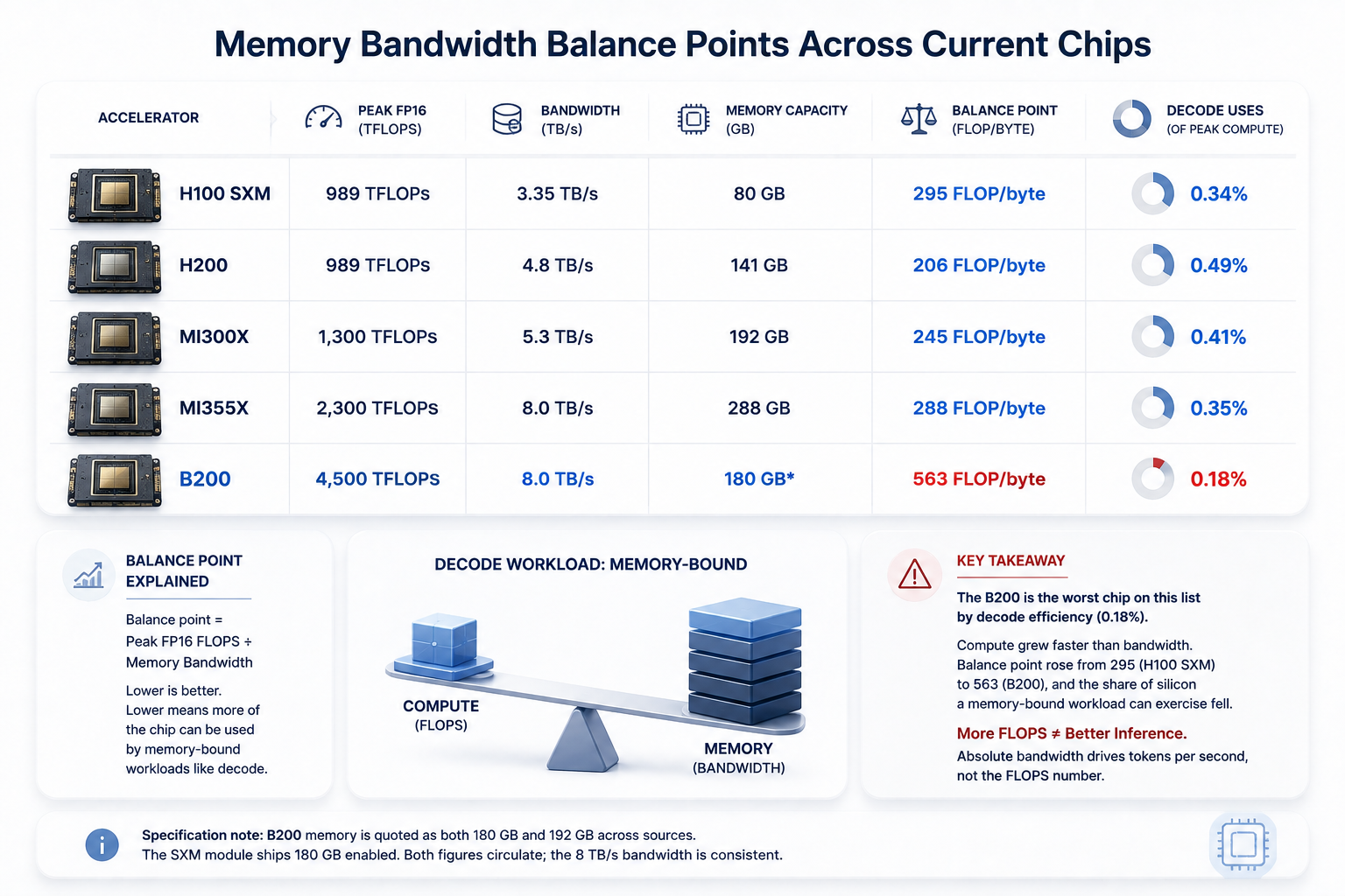
Here is the arithmetic, computed from published specifications. Balance point is peak dense FP16 FLOPS divided by memory bandwidth.

Accelerator	Peak FP16	Bandwidth	Capacity	Balance point	Decode uses
H100 SXM	989 TFLOPS	3.35 TB/s	80 GB	295 FLOP/byte	0.34%
H200	989 TFLOPS	4.8 TB/s	141 GB	206 FLOP/byte	0.49%
MI300X	1,300 TFLOPS	5.3 TB/s	192 GB	245 FLOP/byte	0.41%
MI355X	2,300 TFLOPS	8.0 TB/s	288 GB	288 FLOP/byte	0.35%
B200	4,500 TFLOPS	8.0 TB/s	180 GB	563 FLOP/byte	0.18%

The final column is the fraction of peak compute a decode workload can actually use. Read it twice.

The B200 is the worst chip on this list by that measure. It has 4.5× the FP16 compute of an H100 and 2.4× the bandwidth. Compute grew faster than bandwidth, so the balance point rose from 295 to 563, and the share of silicon a memory-bound workload can exercise fell.

This is not an argument against buying B200s. In absolute terms a B200 generates far more tokens per second than an H100, because absolute bandwidth is what matters for throughput. It is an argument against reading the FLOPS number as a proxy for inference performance. Those two things diverged.

One specification note: B200 memory is quoted as both 180 GB and 192 GB across sources. The SXM module ships 180 GB enabled. Both figures circulate; the 8 TB/s bandwidth is consistent.

---

The H200 Natural Experiment

Theory is arguable. This comparison is not.

The H200 uses the same compute die as the H100. Identical FLOPS. What changed was memory: 80 GB of HBM3 at 3.35 TB/s became 141 GB of HBM3e at 4.8 TB/s.

If FLOPS determined inference performance, the two would perform identically. They do not. MLPerf results using Llama 2 70B showed the H200 exceeding 31,000 tokens per second, roughly 45% faster than the H100.

A 43% bandwidth increase produced roughly a 45% throughput increase, with zero additional compute.

That is close to linear scaling with bandwidth, and it is the clearest available demonstration that memory bandwidth — not compute — governs decode throughput.

One caveat worth carrying into procurement: a 43% throughput gain only lowers your cost per token if the hourly price premium is below 43%. Bandwidth improvements are real, and they are still something you pay for.

---

Calculating Your Token Ceiling From Memory Bandwidth

You can compute an upper bound before running anything.

Tokens per second ≤ memory bandwidth ÷ bytes of weights read per token

At batch size 1, the weights read per token equal the model size in memory. Here is a 70B model across precisions and chips.

Chip	FP16 (140 GB)	FP8 (70 GB)	FP4 (35 GB)
H100	— (does not fit)	48 tok/s	96 tok/s
H200	34 tok/s	69 tok/s	137 tok/s
MI300X	38 tok/s	76 tok/s	151 tok/s
B200	57 tok/s	114 tok/s	229 tok/s
MI355X	57 tok/s	114 tok/s	229 tok/s

These are ceilings, not forecasts. Real throughput lands below them because of kernel launch overhead, imperfect memory access patterns, and attention operations on top of weight streaming.

But the ceiling is genuinely hard. No amount of optimization produces more tokens per second than bandwidth divided by bytes moved.

Two things fall out immediately. Quantisation roughly doubles the ceiling per halving of precision, because it halves the bytes moved. And batching raises aggregate throughput without raising per-request speed, because the same weights serve multiple requests per pass — which is why throughput and latency behave so differently under load, and why cost per token depends so heavily on utilisation.

---

Why the KV Cache Makes Memory Bandwidth Worse

Weight streaming is the headline problem. The KV cache is the one that degrades over a conversation.

Each generated token must retrieve key and value vectors for every preceding token. That traffic grows linearly with sequence length, and the access pattern is irregular in address space.

Irregularity matters more than volume here. HBM delivers rated bandwidth on sequential, row-buffer-friendly access. Scattered reads produce poor row-buffer locality, and effective bandwidth falls well below the rated peak.

So two things happen as context grows. Total bytes moved per token increase, and the efficiency with which they move decreases.

This is why long-context serving degrades faster than a linear model predicts, and why published peak bandwidth is an optimistic upper bound rather than a working number.

FP8 KV cache quantisation is the cheapest available intervention — it halves KV traffic against FP16, and it is usually simpler to deploy than changing hardware.

---

Four Ways to Buy Back Memory Bandwidth

Ordered by effort, not by effect.

Quantise the weights. Moving from FP16 to FP8 halves bytes per token and roughly doubles the ceiling. FP4 halves it again where accuracy holds.

Quantise the KV cache. Separate from weight quantisation and often overlooked. Halves KV traffic.

Batch. Weights are read once and reused across every request in the batch, so arithmetic intensity rises with batch size. This moves the workload up the roofline toward the compute-bound region — the only lever that changes which ceiling binds.

Check your kernels. This is the least obvious and frequently decisive. A 2026 cross-GPU study found that quantisation only delivers bandwidth savings if the kernel actually streams compressed weights through memory. Two int4 implementations on the same hardware differed by more than 2× in step time, with the difference attributable to kernel implementation rather than bit width.

That last finding deserves emphasis. You can quantize a model, halve its nominal footprint, and see no throughput gain, because the runtime dequantises before the bytes cross the memory bus.

---

Where the Memory Bandwidth Model Breaks Down

A model that only confirms itself is not worth trusting. Here is where this one fails.

Rated bandwidth is not achieved bandwidth. Every figure in the tables above is a peak specification. Real workloads see less, sometimes substantially, because of irregular access patterns and row-buffer misses. Treat computed ceilings as upper bounds that real systems approach but do not reach.

Latency and launch overhead are not modelled. A 2026 cross-GPU study found that for small models at batch size 1, kernel launch overhead — not bandwidth — dominated step time. One 7B model reached 11.78 ms per step under default attention with CUDA graphs enabled, a regime where the roofline is not the binding constraint at all. Below roughly 7B parameters at batch 1, check launch overhead before blaming memory.

Interconnect becomes the next wall. Once a model spans multiple accelerators, tensor and expert parallelism push traffic across NVLink or equivalent fabric. Research notes this as the subsequent bottleneck after memory bandwidth and capacity, and large mixture-of-experts deployments are already approaching it.

Mixture-of-experts changes the arithmetic entirely. An MoE model activates a fraction of its parameters per token, so bytes moved per token bear little relation to total parameter count. Substituting total parameters into the ceiling formula will give an answer that is wrong by an order of magnitude.

Cost inversions are real. The same study found that an H100 was roughly 1.47× faster than an L4 on one quantised workload, while costing more than ten times as much per hour. Faster and cheaper-per-token are different questions, and the memory bandwidth ceiling only answers the first.

---

What HBM4 Changes for Memory Bandwidth

HBM4 enters mass production in 2026 and doubles the interface width to 2048 bits while holding transfer rates above 8.0 Gbps, reaching roughly 2 TB/s per stack.

Doubling width rather than clock speed is the important design choice — it raises throughput without a proportional power penalty.

Two things to keep in perspective.

The balance point may not improve. If next-generation compute scales faster than next-generation bandwidth, the gap widens again, exactly as it did from H100 to B200. Bandwidth doubling is only relief if compute does not more than double alongside it.

Supply is the binding constraint. HBM demand grew more than 130% year over year in 2025 and is projected above 70% in 2026. Memory availability now determines which organisations can deploy the largest models, which is a supply-chain fact rather than an engineering one.

---

Reading Memory Bandwidth Claims Critically

A short checklist for vendor material.

Find the precision. A FLOPS figure without a precision is meaningless. FP4 numbers are typically 4× the FP16 figure for the same silicon.

Check dense versus sparse. Sparse figures typically double dense ones and require structured sparsity your model may not have.

Divide FLOPS by bandwidth yourself. That single division tells you more about inference behavior than any headline throughput claim.

Ask which phase was measured. Prefill-heavy benchmarks flatter compute. Decode-heavy benchmarks reveal bandwidth.

Treat vendor comparisons as workload-specific. One current marketing claim compares a liquid-cooled part at FP4 against a prior-generation part at FP8 under different batch conditions. That is not a like-for-like measurement, and the same pattern recurs across vendors.

Watch for capacity-bandwidth conflation. More memory lets you fit a larger model. It does not make token generation faster. The MI355X’s 288 GB is a capacity advantage; its 8 TB/s is the throughput number.

Terminology in this area is inconsistent across vendors, and our AI glossary defines the specific terms used here.

---

Primary sources

• Williams, Waterman & Patterson, Roofline model (ACM)
• NVIDIA data centre GPU specifications
• AMD Instinct MI350 series
• TrendForce memory wall analysis

Balance points and token ceilings above are computed from published vendor specifications using the formulas shown, so readers can substitute their own figures. Vendor capacity figures occasionally conflict; discrepancies are noted inline.

---

Frequently Asked Questions

---

Keep reading

Here are the latest posts from the blog.