inference benchmarking

Published October 2026 · Data read October 11, 2026 · Source: Artificial Analysis provider benchmarks, secondary research

The same open-weight model, Llama 3.3 70B, starts answering in 0.67 seconds on Google Vertex and 2.37 seconds on DeepInfra. Once it starts, Groq streams 328 tokens per second and DeepInfra 17. A 500-token answer takes 2.4 seconds on Groq and 32.5 seconds on DeepInfra’s FP8 “Turbo” endpoint.

Those figures come from Artificial Analysis, which runs the same 10,000-token prompt against every host from one Google Cloud VM in Iowa and reports the median over 72 hours. That is about as fair as public LLM inference latency data gets, and it is still not perfectly fair. DeepInfra’s endpoint is quantized to FP8, no host discloses its hardware or batch size, and a request from Frankfurt or Mumbai will see different network time.

The spread is the point. Rate limits tell you how much a provider lets you run, and pricing tells you what it costs. Latency decides whether the product feels usable. That depends far more on the serving stack and the settings you choose than on the model’s name.

Key Takeaways

• For one model, host choice moved output speed 19-fold (17 to 328 tokens/s for Llama 3.3 70B) and time to first token 3.5-fold.
• Reasoning effort dominates frontier-model latency. On Artificial Analysis’s default “max” setting, Claude Sonnet 5.5 took about 490 seconds to its first answer token. Its low setting is listed at under a second on the provider leaderboard, a figure to check before quoting.
• Time to first token (TTFT) and output speed are separate problems. A short chat reply is dominated by TTFT. A long report is dominated by output speed.
• Agents multiply latency. Five sequential calls on a slow endpoint can take more than 100 seconds before tool time is added.
• Published medians hide tail latency. No source examined here published p95 figures, so you have to measure them yourself.
• Test with your own prompt lengths, region and reasoning settings before trusting any ranking, including this one.

---

Quick Navigation

---

Why LLM inference latency is hard to compare

Two published numbers for “the same model” can differ for at least six reasons that have nothing to do with the model: where the test client sits, how long the prompt is, how many requests run at once, which reasoning setting is on, how the host quantizes and batches, and which statistic is reported.

Even one careful source can disagree with itself. On Artificial Analysis’s Gemini 3.5 Flash-Lite page, the headline gives 414 tokens per second and the comparison table gives 365. Its GPT-6.1 Sol page reports a time to first answer token of 311 seconds in the headline and 327 seconds in the table. Neither page explains the gap. Different averaging windows are the likely cause, but that is an inference, not a documented fact. If a single benchmark cannot hold one number steady across its own page, rankings stitched together from several sources deserve more suspicion.

What TTFT actually measures

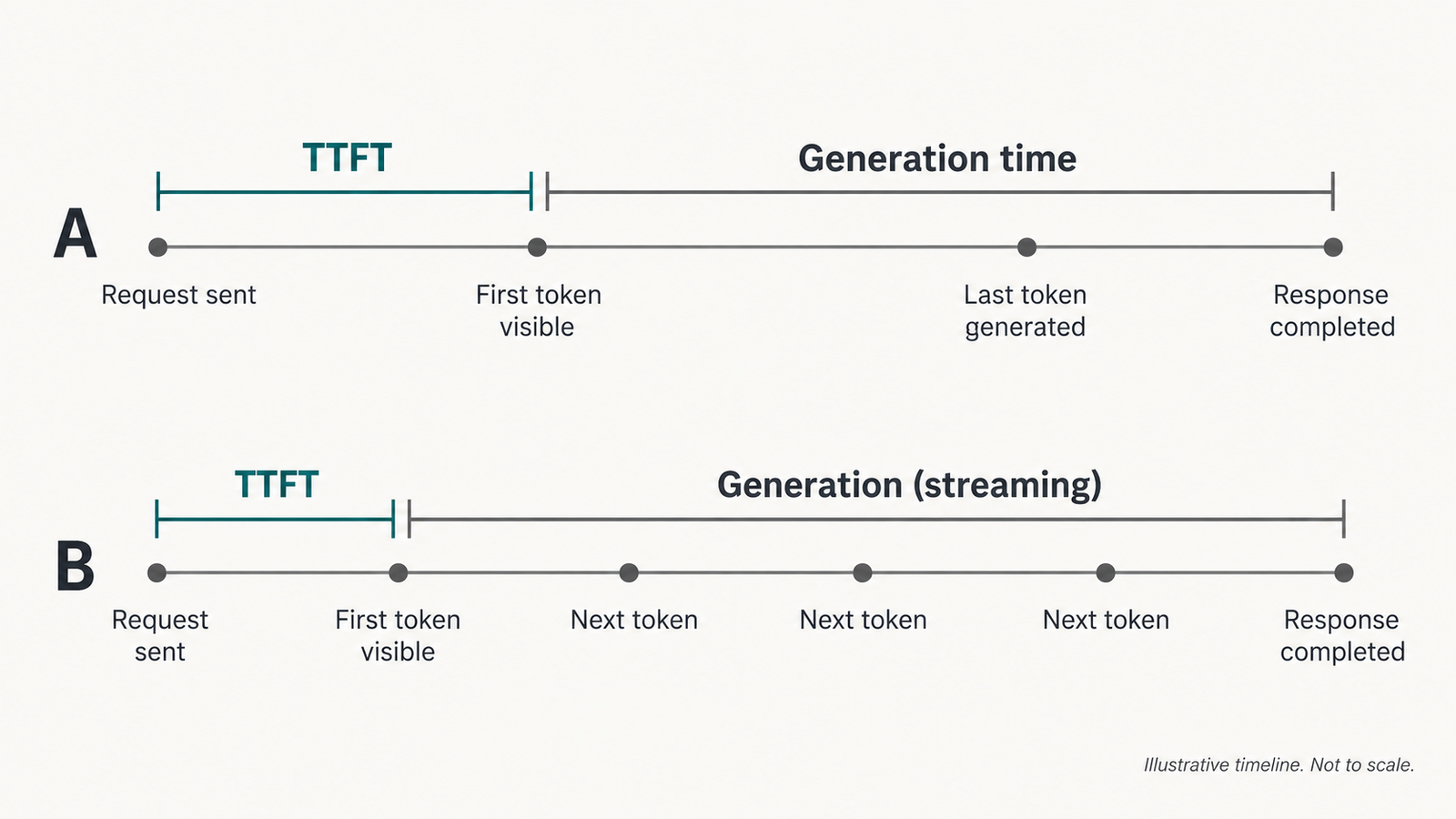
Time to first token (TTFT) is the wall-clock time between sending a request and receiving the first token of the response. Artificial Analysis’s methodology defines it that way and measures from the client.

That single number folds together several stages:

• network time from client to provider and back
• admission and queueing behind other customers’ requests
• prefill, where the model processes the entire prompt before it can generate anything
• any provider-side orchestration, such as safety checks, routing or tool-schema handling
• for reasoning models, the thinking phase, if the measurement waits for the first answer token

Providers do not publish this breakdown, and a client-side measurement cannot separate the stages. A slow TTFT could mean a long queue, a long prompt or a distant data centre.

The reasoning point causes most of the confusion. Artificial Analysis reports two variants: TTFT to the first token of any kind, and “time to first answer token”, which includes thinking. Its per-model pages for frontier models use the second variant. That is why Claude Opus 5.5 at max effort shows roughly 600 to 1,000 seconds depending on host. The figure measures how long the model chose to think, not how fast Anthropic, Google, Azure or Amazon serve it.

TTFT versus output tokens per second

Output speed is the average rate at which tokens arrive after the first one. Artificial Analysis defines it as tokens received per second after the first token. It governs how long a full answer takes. TTFT governs how long the user stares at nothing.

The two do not move together. On Llama 3.3 70B, Google Vertex had the lowest TTFT (0.67 s) but streamed at 162 tokens/s, while SambaNova was slower to start (2.26 s) but generated faster (280 tokens/s). For a 50-token reply, Vertex wins comfortably. For a 2,000-token document, SambaNova finishes first.

The gap comes from different bottlenecks. Prefill is mostly compute-bound, processing many prompt tokens in parallel. Decode, the token-by-token generation that follows, is mostly limited by memory bandwidth, because the model’s weights stream through the chip for every token. Hardware and batching choices that help one phase can hurt the other. Large batches raise a provider’s total throughput but slow each individual stream.

LLM inference latency by model and provider

All figures are third-party measurements by Artificial Analysis, read October 11, 2026. Conditions throughout: about 10,000 input tokens, single request at a time, client in Google Cloud us-central1-a, streaming, median of the previous 72 hours. “End-to-end” is the time to receive a 500-token answer. None of this was measured by UniverseBlend.

Table 1: One model, many hosts (the controlled comparison)

Model	Host	TTFT (s)	Output speed (tok/s)	End-to-end, 500 tokens (s)	Notes
Llama 3.3 70B	Google Vertex	0.67	162	3.76	Precision not reported
Llama 3.3 70B	Groq	0.85	328	2.37	Custom LPU hardware
Llama 3.3 70B	CoreWeave	0.89	78	7.34	Not reported
Llama 3.3 70B	Scaleway	1.48	73	8.34	Headline TTFT 1.34 s
Llama 3.3 70B	Together AI (Turbo)	1.59	71	8.65	“Turbo” variant
Llama 3.3 70B	Novita	1.78	45	12.83	Not reported
Llama 3.3 70B	Azure	2.24	121	6.38	Not reported
Llama 3.3 70B	SambaNova	2.26	280	4.05	Headline speed 294.5
Llama 3.3 70B	DeepInfra (Turbo)	2.37	17	32.53	FP8
Llama 3.3 70B	Parasail	2.57	86	8.39	FP8

Source: Artificial Analysis, Llama 3.3 70B providers. p95: not reported for any row.

Table 2: Frontier models at maximum reasoning effort

Model (API ID)	Host	Time to first answer token (s)	Output speed (tok/s)	End-to-end, 500 tokens (s)
Claude Sonnet 5.5 (claude-sonnet-5-5)	Amazon	475.97	143	479.46
Claude Sonnet 5.5	Anthropic	492.88	142	496.41
Claude Opus 5.5 (claude-opus-5-5)	Google	604.25	95	661.24
Claude Opus 5.5	Anthropic	704.18	97	667.28
GPT-6.1 Sol (gpt-6.1-sol)	Azure	288.60	78	294.99
GPT-6.1 Sol	OpenAI	326.94	56	335.94

Sources: Artificial Analysis provider pages for Claude Sonnet 5.5, Claude Opus 5.5 and GPT-6.1 Sol. Effort: “max” with default fallback (Claude); “max” (GPT-6.1 Sol). These numbers mostly measure thinking time. Several Opus 5.5 rows show a time-to-first-answer longer than the 500-token total, an inconsistency the source does not explain.

Table 3: Lower-effort and lightweight endpoints (leaderboard view)

Model	Host	First chunk (s)	Output speed (tok/s)	Total (s)	Setting
Claude Sonnet 5.5	Anthropic	0.88	100	5.86	low effort
GPT-6 Luna (gpt-6-luna)	OpenAI	2.83	125	6.84	low effort
GPT-6.1 Sol	OpenAI	2.80	47	13.41	low effort
Gemini 3.5 Flash-Lite (gemini-3.5-flash-lite)	Google AI Studio	8.96	365	10.33	default; reasoning not reported
Qwen3.8 2.4T A95B	Together AI	1.14	112	23.40	not reported
Qwen3.8 2.4T A95B	DigitalOcean	0.82	57	44.54	not reported
Qwen3.8 2.4T A95B	Alibaba Cloud	2.99	37	71.44	not reported

Source: Artificial Analysis provider leaderboard, with Gemini from its model page. Treat this table as indicative: column values were extracted from a combined view and should be confirmed on the live page. The Qwen totals are high relative to their speed, which suggests reasoning output or longer answers. The source does not say which.

The Sonnet 5.5 rows across Tables 2 and 3 tell the main story. The same model on the same host goes from under one second to about eight minutes before answering, depending on a single API parameter.

Measurement-quality matrix

Comparison	Same model?	Same harness?	Same settings?	Verdict
Llama 3.3 70B across hosts (Table 1)	Yes	Yes	Precision varies	Controlled; fair to rank, noting FP8 rows
One frontier model across clouds (Table 2)	Yes	Yes	Yes (max effort)	Partially comparable; differences mix serving and thinking-time variance
Different frontier models (Table 2)	No	Yes	Effort labels differ by vendor	Unsuitable for a speed ranking; effort levels are not equivalent across vendors
Low-effort rows (Table 3)	No	Yes	Varies	Indicative only
Qwen across hosts (Table 3)	Yes	Yes	Not reported	Partially comparable
Any of the above versus your own region and concurrency	n/a	No	No	Unsuitable without retesting

How prompt length changes the first-token experience

Before a model can write its first word, it has to process every prompt token. More input means more prefill work, so TTFT generally rises with prompt length. Attention also scales worse than linearly with sequence length, which matters most at very long contexts.

In production the relationship is rarely clean. Providers split long prompts into chunks, interleave them with other customers’ work, and route long-context requests to different hardware. Artificial Analysis tests at 1,000, 10,000 and 100,000 input tokens for this reason. All the figures above use the 10,000-token workload, so they overstate TTFT for a short chat turn and understate it for a large retrieval prompt.

Caching changes the picture for repeated prefixes. Anthropic’s prompt-caching documentation says users “will generally see improved time-to-first-token for long documents” when a cached prefix is reused. Caching has no effect on output generation, and the default cache lives five minutes. The documentation gives no millisecond figure, so measure the gain on your own prompts.

Typical input size	What to measure beyond the published median
Under 2,000 tokens (chat turns, classification)	TTFT and first visible text from your own region; p95 under expected concurrency
2,000–30,000 tokens (RAG, documents)	TTFT at three or more sizes in this range; cache-hit versus cache-miss TTFT
30,000+ tokens (codebases, long files)	TTFT growth curve up to your real maximum; timeouts and error rate; whether the endpoint routes long prompts differently
Any size with a fixed system prompt	Cached-prefix TTFT, and how quickly the cache expires under your traffic pattern

When streaming helps and when it does not

Streaming sends tokens as they are generated instead of waiting for the full response. It does not make the model faster. It changes when the user first sees something.

For a chat interface, that is often enough. Jakob Nielsen’s widely cited response-time limits, drawn from Miller (1968) and Card et al. (1991), put the edge of uninterrupted thought at about one second and the edge of sustained attention at about ten. A streamed answer that starts within a second and reads at a steady pace keeps a reader engaged, even if completion takes eight seconds.

Streaming fails in three common cases. The first is when the client needs the whole response before acting: structured JSON, a tool call or a function argument cannot be used half-written. The second is uneven cadence. Long pauses mid-stream, from server batching or client buffering in proxies and UI frameworks, can feel worse than a slightly later start. The third is reasoning models that show nothing until thinking ends, so a fast first token is meaningless if that token is hidden reasoning.

What LLM inference latency means for AI agents

This is where latency stops being a benchmark number and becomes a product problem. An agent rarely makes one call. It plans, calls a tool, reads the result and calls the model again, and every step pays TTFT and generation time in sequence.

A rough estimate per step:

T_{\text{step}} \approx \text{TTFT} + \frac{\text{output tokens}}{\text{output tokens per second}} + T_{\text{tool}}

This is an approximation. It ignores mid-stream pauses, retries and queueing spikes, and it assumes steps run one after another rather than overlapping.

The formula reproduces the source’s own totals. For Groq, 0.85 s + 500 / 328 tok/s = 2.37 s, exactly the published end-to-end figure. For DeepInfra, 2.37 + 500 / 17 = 31.8 s, against 32.5 s published.

Worked example (derived, not measured): a five-step agent, each step producing 300 output tokens and making one tool call that takes an assumed 0.8 seconds.

Endpoint (Table 1 or 2 figures)	Per step	Five steps
Llama 3.3 70B on Groq	0.85 + 0.91 + 0.8 = 2.56 s	12.8 s
Llama 3.3 70B on Google Vertex	0.67 + 1.85 + 0.8 = 3.32 s	16.6 s
Llama 3.3 70B on DeepInfra (FP8)	2.37 + 17.65 + 0.8 = 20.82 s	104 s
Claude Sonnet 5.5, max effort, Anthropic	492.88 + 2.11 + 0.8 = 495.8 s	about 41 minutes

The same five-step task is a 13-second interaction or a 41-minute background job, depending on host and settings. Neither outcome is wrong, but each implies a different product. Voice is stricter still: Stivers et al.’s 2009 PNAS study of turn-taking across 10 languages found average gaps between speakers clustering within 250 milliseconds of a cross-language mean. That points to a budget measured in hundreds of milliseconds, not seconds. That figure is a design guide drawn from human conversation, not a measured LLM threshold.

A reasonable set of engineering guidelines, labelled as such: aim for first visible text under about one second in chat, under a few hundred milliseconds of response gap in voice, and set an explicit end-to-end budget for agents, with p95 rather than median as the target.

Hosted APIs versus Llama and Qwen inference hosts

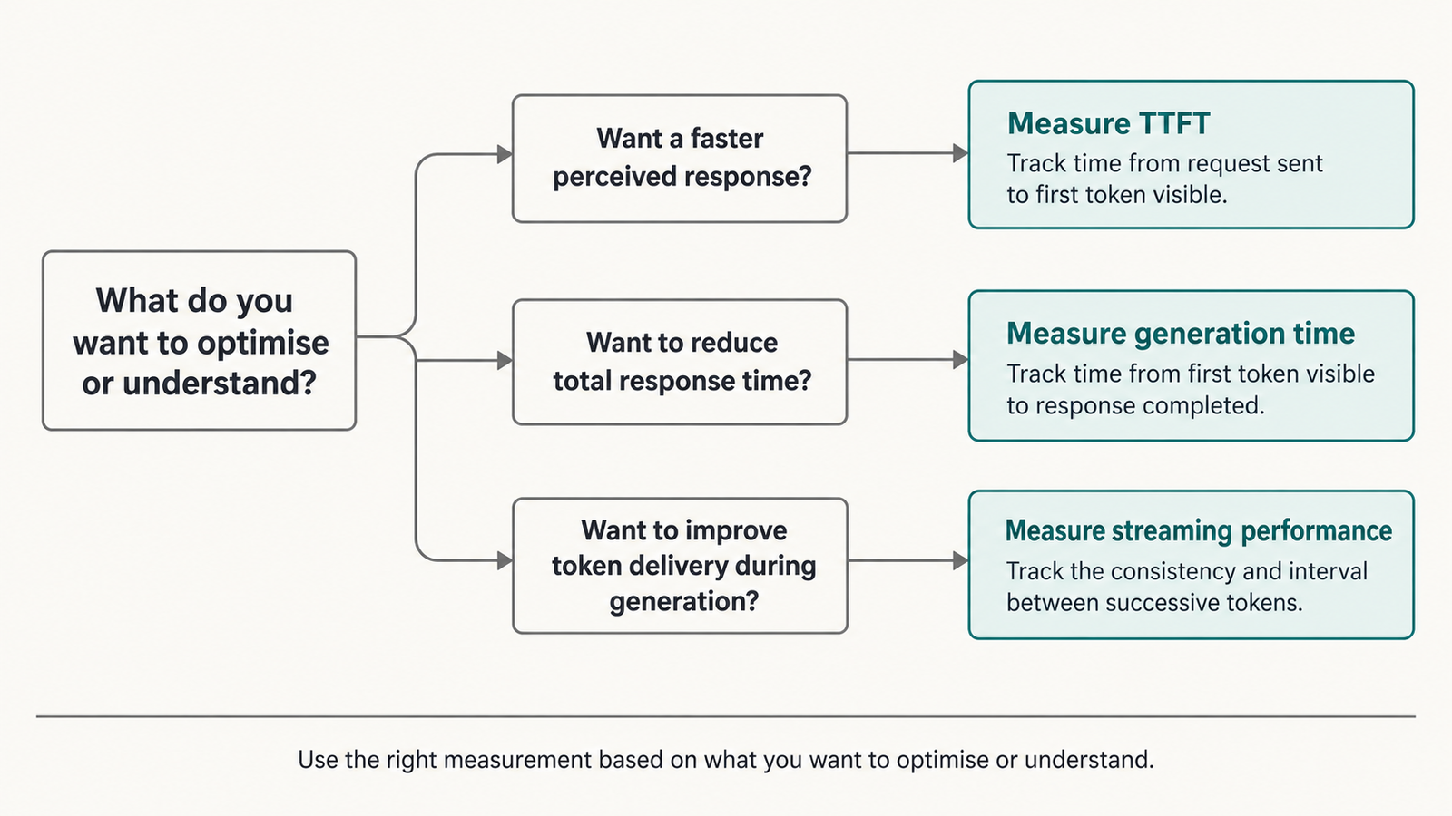
With a closed model, you can only buy latency from the vendor or the clouds that resell it. Table 2 shows that resellers can differ: GPT-6.1 Sol reached its first answer about 38 seconds sooner on Azure than on OpenAI’s own API, and streamed faster. With open weights you can also choose the serving stack, and Table 1 shows that choice matters more than anything else measured here.

That difference belongs to the host, not the model. Llama 3.3 70B is identical weights everywhere, yet output speed varies 19-fold. The causes are mostly undisclosed: accelerator type (Groq and SambaNova build their own chips), quantization (DeepInfra and Parasail are FP8), batch size and scheduling policy, and data-centre location relative to the test client. A slow host is not evidence that the model is slow, and a fast host’s numbers do not transfer to your own deployment.

Self-hosting gives you control of those variables and the responsibility for tuning them. It is also the economic question UniverseBlend examined in GPU Cloud Pricing 2026. Larger batches lower cost per token and raise per-request latency, so the cheapest configuration is rarely the most responsive one.

How to run a fair LLM inference latency test

No public benchmark matches your region, prompts and traffic. A minimal test you can run yourself:

1. Run the client in the cloud region your users or servers actually use.
2. Build prompts at your real input sizes, with three lengths minimum, and unique content per request so caching does not flatter results (then test cached prefixes separately).
3. Fix output length with max_tokens and record the actual tokens returned.
4. Set reasoning effort, temperature and tool schemas exactly as production will.
5. Stream every request and timestamp each chunk on the client.
6. Run at least a few hundred requests per configuration, spread across days and hours, at your expected concurrency.
7. Report p50 and p95 for TTFT, inter-token gap and total time, plus the error and timeout rate.

import time

def measure(client, prompt, **settings):
    t0 = time.perf_counter()
    stamps = []
    for chunk in client.stream(prompt, **settings):   # provider SDK streaming call
        if chunk.text:                                  # ignore empty/keep-alive chunks
            stamps.append(time.perf_counter())
    ttft = stamps[0] - t0
    gaps = [b - a for a, b in zip(stamps, stamps[1:])]
    total = stamps[-1] - t0
    return {"ttft": ttft, "total": total,
            "max_gap": max(gaps, default=0),
            "chunks": len(stamps)}
# Run many times; report p50/p95 of each field, not the mean.

Chunks are not always single tokens, so divide counted output tokens by streaming time for a true rate. This sketch produces no results by itself, and none are reported here.

A practical provider selection framework

Pick metrics by workload before comparing providers.

Criterion	Matters most when	How to judge
TTFT at your input size	Chat, autocomplete, voice	p95 from your region
Sustained output speed	Long answers, reports, code	Tokens per second after the first token
End-to-end completion	Anything parsed as a whole (JSON, tools)	p50 and p95 total time
Variability	User-facing products	Gap between p50 and p95; largest mid-stream pause
Concurrency and rate limits	Production traffic	Latency at expected parallelism; see AI API rate limits in 2026
Tool-call overhead	Agents	Per-step time multiplied by expected steps
Cost at required quality	All	Cost per completed task at the reasoning setting you need

A single fastest-model ranking misleads in both directions. It can reward an endpoint that is fast because it thinks less, and penalise a model whose latency comes from a reasoning setting you would never use. Fix quality first, then compare latency among the options that meet it.

What the available evidence cannot tell us

The public data has clear gaps. It has no tail latency (medians only), one client location, mostly single-request load, and undisclosed hardware and batch sizes. Reasoning effort labels mean different things at different vendors. Frontier-model pages default to maximum effort, which few interactive products would use. Several source pages also show internal inconsistencies, so any figure here could shift by 10% or more when re-read. None of it tells you how a provider behaves during a regional incident or a demand spike, which is when latency matters most.

Conclusion

LLM inference latency becomes a product problem at a specific point: when the time a user or a downstream system must wait crosses the budget your interface was designed around. For chat that is roughly a second to first visible text. For voice it is hundreds of milliseconds. For agents it is the sum of every step, at the 95th percentile.

The evidence says the model name predicts that wait poorly. Host choice moved Llama 3.3 70B’s output speed 19-fold, and one reasoning parameter moved Claude Sonnet 5.5 from under a second to about eight minutes. Treat published rankings as a shortlist, then measure the two or three candidates yourself, with your prompts, in your region, at your load.

Frequently Asked Questions

What is a good LLM inference latency for a chatbot?

There is no universal standard. A common engineering guideline, based on Nielsen’s one-second limit for uninterrupted thought, is first visible text within about one second, with steady streaming after that. Measure p95, not just the median.

What is time to first token (TTFT)?

TTFT is the time from sending a request to receiving the first token of the response, measured at the client. It includes network time, queueing and prompt processing. For reasoning models it may also include thinking time, depending on whether the measurement waits for the first answer token.

Is TTFT or output tokens per second more important?

It depends on response length. Short replies are dominated by TTFT, and long documents by output speed. Estimate total time as TTFT plus output tokens divided by output speed for your typical response.

Why does the same open model have different latency on different hosts?

Hosts use different hardware, quantization, batching and data-centre locations. On Artificial Analysis’s October 2026 data, Llama 3.3 70B ran at 17 to 328 output tokens per second depending on host.

Why do reasoning models seem so slow in benchmarks?

Many benchmarks report time to the first answer token at the highest reasoning effort, which includes minutes of thinking. Lower effort settings respond in seconds. Compare models at the effort level you would actually use.

Does streaming reduce latency?

Streaming reduces the time until users see output, not the time to generate the full response. It helps chat, but does nothing for tool calls or structured output that must arrive complete.

Does prompt caching reduce latency?

It can reduce TTFT when a long prompt prefix repeats. Anthropic documents improved time-to-first-token for long cached documents and no effect on output generation speed. Gains depend on cache hits within the cache lifetime.

How do I benchmark LLM inference latency fairly?

Test from your production region, with your real prompt sizes and settings, streaming, at expected concurrency, over hundreds of requests across several days. Report p50 and p95 for TTFT and total time, plus errors.

---

Keep reading

Here are the latest posts from the blog.