Tech

I’m seeing Claude local deployment edge computing AI tools coming up as one of the hottest topics in developer Slack groups and IT forums. And really? We can understand why. Faster inference, better privacy, reduced long term expenses – what’s not to like? However, running large language models (LLMs) locally is not just a matter of downloading a file and clicking “run.” I’ve watched a lot of teams learn that the hard way.

The emergence of edge computing has altered the way enterprises approach AI infrastructure. More specifically, teams now have a true architectural option to make: do we retain LLM workloads in the cloud, or push them closer to the people that require them? This guide cuts through the marketing hype and explains the real trade-offs.

If you’re designing offline-first applications or trying to shave milliseconds off latency-sensitive activities, understanding deployment topology matters more than any feature checklist. This insight is moreover directly useful for systems such as Claudemesh, where local sessions depend on an underlying reliable infrastructure layer.

Why Claude Local Deployment Edge Computing AI Tools Matter Now

Three drivers are driving the trend to local AI inference. And they’re not slowing down.

Privacy regulations are getting tougher. Healthcare, finance, government – these industries don’t always have the ability to route sensitive data to other servers. So organisations require models that can be run on their own premises. And, with the General Data Protection Regulation (GDPR) and related regulations, cloud-only deployments have become truly hazardous for sensitive workloads. This startled me when I first started researching into compliance standards – the legal risk is more significant than most developers first anticipate. A midsize radiology firm I spoke with had quietly abandoned a cloud-based AI triage tool after their legal team raised concerns about patient imaging metadata being shared to a third party’s server. They got the workflow running locally in approximately 3 months, and never looked back.

Latency kills the user experience. Cloud round-trips add 50-200ms overhead each request. Meanwhile, edge inference can provide responses in single-digit milliseconds for smaller models. That difference counts a lot for real-time applications such as coding assistants and customer-facing chatbots. I’ve tested many dozens of configurations and users definitely sense the difference, even if they can’t explain why one is “snappier”. In one informal test with a customer service team, agents rated the local inference tool 23% higher on “responsiveness” without ever being told which backend was powering each session.

Cloud costs can add up rapidly. API pricing is useful for prototyping. But at scale, the costs per token build up quickly. A team generating 100,000 API calls per day can easily burn through thousands per month. Local deployment transforms that reoccurring expense into a one-time hardware purchase. The math isn’t always straightforward to start with, but it soon becomes clear. A good activity is to take the last three months of your API invoices and plot cost against request volume. The slope of the line informs you exactly how urgently you should be thinking about local alternatives.

Additionally, Claude local deployment edge computing AI solutions allow teams to have complete control over model versioning. You don’t wake up to a sudden model update that ruins your process. “Honestly, the best part is you can upgrade at your own pace. I have watched production pipelines break overnight because a cloud provider changed tokenization behavior with no fanfare. When you own the stack, this is not the case.

But in practice it is more complicated. Unlike Meta’s Llama, Anthropic does not release the weights for Claude so that you can self-host. “Local Claude deployment” generally indicates one of the following approaches:

• Use the Anthropic API to run Claude with local caching layers
• Using a distillation or fine-tuned open model that mimics the behavior of Claude
• Using hybrid architectures in which edge devices are used for pre-processing and the cloud for complicated inference
• Claudemesh style session management for offline-capable workflows

Edge Devices vs Cloud: A Direct Comparison for AI Deployment

The Edge vs. Cloud deployment is not a black or white choice. Most production methods are a mixture. But knowing the raw differences helps you create the correct architecture — so here’s the honest breakdown.

Factor	Edge / Local Deployment	Cloud Deployment
Latency	1–10ms (on-device)	50–300ms (network-dependent)
Privacy	Data stays on-premise	Data transits to third-party servers
Upfront cost	High (GPU hardware)	Low (pay-as-you-go)
Ongoing cost	Electricity + maintenance	Per-token or per-request fees
Model size support	Limited by local RAM/VRAM	Virtually unlimited
Scalability	Manual hardware provisioning	Instant auto-scaling
Offline capability	Full functionality	None without connectivity
Model updates	Manual deployment required	Automatic from provider

“Hardware is the largest bottleneck for edge computing AI tools,” he said. Take Claude 3.5 Sonnet for example – a huge model — executing it locally at full precision would require enterprise-grade GPUs most organizations just don’t have lying around. But you can run quantized or distilled versions on more basic hardware, but you’re trading quality to get there. Fair warning: the trade-off is worse for sophisticated reasoning tasks than simple ones. A quantized model can crush “summarize this support ticket” but fumble at “identify the root cause across these 40 interrelated log entries”.

The cost crossover point. Local deployment is cheaper than cloud for most teams at some 50,000–100,000 daily requests. Below this threshold, cloud APIs generally win on total cost of ownership. Own your hardware and it begins to make some serious financial sense above it. One tip: Don’t just count your present request volume, project it 12 months out. Teams that hit that milestone six months into a project sometimes wish they’d started out with the hardware.

Hybrid is often the answer. Smart architectures can direct simple queries to local models and sophisticated queries to the cloud. Tools like NVIDIA Jetson are also making edge AI technology more accessible than ever before, and that gap keeps becoming smaller.

Setting Up Claude Local Deployment: Practical Architecture Patterns

These are the most viable patterns for production deployment of Claude local edge computing AI technologies. I’ve seen all of these work nicely, in the correct setting.

1. API gateway with local caching. This is the easiest way, and frankly a good way to start. You set up a local proxy that caches common replies from the Claude API. New queries still hit Anthropic’s cloud, but repeated inquiries can be answered locally immediately. This is especially useful for customer service bots because the questions are predictable – one organization I spoke to saved 40% on their API charges with this method alone. The tradeoff is staleness: cached responses do not know about model changes or updated information, hence a smart cache invalidation policy is needed. Good time-to-live numbers for most support use cases are between 24 and 72 hours.

2. Edge preprocessing with cloud inference. Tokenization, context assembly and input validation are performed on your local device. The last prompt goes only to the cloud, which decreases payload size and improves perceived latency. Response post-processing is also done locally, so sensitive output transformations remain on-premise. It’s a clever compromise. One real-world example: a legal tech team utilized this pattern to extract personally identifying information (PII) from documents before to sending them for cloud inference and then re-insert the PII into the final output locally. Their compliance team approved it in a week – something that had been rejected for months under a pure cloud approach.

3. Distilled model deployment. Then you train a smaller model to match Claude’s behavior in your unique use case, and run the distilled model completely on edge hardware. It won’t be as capable as Claude, but it can do 80-90% of domain-specific queries rather effectively. Hugging Face has thousands of models that are good places to start with distillation. The real issue is the upfront cost — distillation takes actual time and expertise to perform right. It will take at least four to eight weeks to make the first meaningful attempt, including review and iteration. Teams who skip this stage usually wind up with a model that works well on their test set but does not perform well on live traffic.

4. Claudemesh session architecture. This approach uses local session management to keep the conversational state on the device. The infrastructure layer deals with context windows, memory management and failover logic. If connectivity exists, sessions synchronize to cloud resources. If not, the local layer continues to work. For apps that are built to work offline initially, such as field service workers in locations with patchy connectivity or clinical instruments in rural hospitals, this is basically a no-brainer.

Hardware considerations for local deployment:

• RAM: Minimum 32GB for quantized 7B parameter models. 64GB+ is strongly recommended if you want headroom.
• GPU VRAM: 24GB handles most quantized models. 48GB+ for larger variants.
• Storage: NVMe SSDs for fast model loading — budget 20–50GB per model.
• CPU: Modern multi-core processors with AVX-512 support meaningfully improve CPU-only inference.

So what deployment strategy is even possible is directly dictated by your hardware budget. Patterns 1 and 2 are easily handled on a $3,000 work station. Patterns 3 and 4 may require $10,000+ worth of dedicated gear Get ready for it.

Privacy, Security, and Compliance in Edge AI Deployments

Privacy is usually the key reason teams begin to look into Claude local deployment edge computing AI products. But here’s the thing: local deployment comes with its own security challenges that cloud deployments don’t have. It’s not a free pass.

The benefits of data residency are genuine. Data never leaves your network – models are executed on your hardware. This meets most data residency criteria. This is a major advantage for firms subject to HIPAA or SOC 2 compliance. And it’s easy to understand why. Healthcare and financial services companies are the top adopters of edge AI.

But model security risks are yours to own. When you host a model locally, it’s your security to manage. You need to guard specifically against:

• Theft or extraction of model weight
• Attacks by adversarial input
• Unauthorized access to inference endpoint
• Side channel attacks on GPU memory

A practical first step: Treat your inference endpoint like you would your internal database. Put it behind your VPN, require mTLS for service-to-service communications, and log each request with a unique trace ID. These are not unusual methods, they are normal backend hygiene applied to a new surface area.

Worries about the supply chain are underestimated. But when you download open-source models for local deployment, you’re trusting the source. Malicious model weights have been seen in the wild – this is not theoretical. Always check checksums and use reputable repositories. Just a heads up, this step is skipped more often than it should be. Add checksum verification to your deployment process so it can’t be unintentionally skipped under deadline constraint.

Audit and logging don’t run themselves. Cloud providers do this for you automatically. You construct your own locally. Regulatory audits also require complete logs of model inputs, outputs and access patterns. Don’t try to glue together a logging system after you’re already in production – think it through before you go live. Most audit needs are met with a structured logging schema that captures the timestamp, user id, prompt hash, answer hash, latency, and model version without keeping sensitive content in plaintext.

Encryption in transit and at rest Encrypt everything, even on local networks. Model weights, discussion logs, cached responses – all must be protected. Use hardware security modules (HSMs) for key management in regulated contexts. If you have sensitive data this is a no-brainer.

The bottom line is that on-premises deployment improves data privacy but raises your security responsibilities. You are trading one set of hazards for another. Moreover, edge computing AI technologies demand continuous security management that would otherwise be taken care of by cloud providers. Ensure your team has the capacity for that before you commit.

Optimizing Performance and Cost for Local Claude Workflows

Running locally requires careful optimization of LLMs. Otherwise you’ll be left with sluggish inference and a wasted hardware investment. But here’s how to truly obtain value from your Claude local deployment edge computing AI tools configuration.

Quantization is your buddy. Moving model weights from 32-bit to 8-bit or 4-bit precision reduces memory requirements considerably. Tools such as llama.cpp make quantizing easier than you think. A model that needs 48GB at full accuracy may need only 12GB at 4-bit. Quality is a little lower but most folks can’t detect the difference for everyday stuff. I was shocked when I first tried it – the gap in quality is much lower than I imagined. The exception is activities that need exact numerical reasoning or multi-step logical chains, where 4-bit quantization could cause small inaccuracies that accumulate over the steps.

Batch inference is resource-efficient. Batch requests together instead of processing them one at a time. In particular, batching can enhance throughput by 3-5x on current GPUs. And that’s not a rounding error, that’s a fundamental difference in efficiency how you employ pricey gear. For asynchronous operations like as document processing or nightly report generation, batching is nearly always the proper thing to do. For interactive use cases, you will need to balance batch size with acceptable wait time – a batch of 10 queries with a 200ms fill window is frequently a good starting point.

Most teams don’t appreciate the importance of managing the context window. Larger context windows use much more memory and slow down inference considerably. Trim unnecessary context aggressively and use summarization to compress conversation history. This one optimization can frequently yield the highest performance increases of anything on this list. One team cut their average context length by 35% just by deleting boilerplate system prompt wording they’d copied from an early prototype and forgotten to revisit.

Selection of task complexity model. Not every inquiry requires your largest model. Send easy categorization tasks to little models, reserve heavyweight inference for complicated reasoning. This tiered technique greatly reduces average inference costs and is the type of improvement that seems simple in retrospect, yet is continuously overlooked. A simple rule of thumb: if a 3B model can get the right answer 95% of the time, sending it to a 70B model is just dead weight.

Cost optimization checklist:

• Keep an eye on GPU usage everyday. > 60% suggests you’re spending too much for hardware.
• If employing cloud GPUs, use spot instances for non-critical batch processing.
• Configure request de-duplication to prevent redundant inference on identical queries.
• Cache embeddings and intermediary calculations if feasible.
• Schedule model loading to prevent cold start penalties during busy hours.
• Track cost-per-query across local and cloud paths so you can compare apples to apples.

One important thing to do is to measure everything because you can’t optimize what you don’t measure. Create dashboards for latency percentiles, throughput, error rates and cost per query Prometheus together with Grafana is a good fit for this monitoring stack. I’ve watched teams skip this step and spend months optimizing the incorrect item. A acceptable minimum viable dashboard: p50, p95 and p99 latency, requests per second, GPU memory consumption and estimated cost per 1000 inquiries. There’s plenty of signal to catch most problems early on.

Conclusion

The local deployment of Claude’s edge computing AI tools is a significant shift in the way that teams construct AI systems. And the difference between edge and cloud isn’t about choosing a winner, it’s about knowing your restrictions and designing around them honestly.

Start by assessing your actual needs. How sensitive is your data?” How much latency will users tolerate? What is your current monthly API spend? Those answers will get you to the correct deployment topology sooner than any framework comparison will.

For most teams, the hybrid approach is preferable. Use local infrastructure for privacy sensitive pre-processing and cached answers. Leverage cloud APIs for complicated reasoning tasks that require the full power of Claude. Also, invest in monitoring from the outset so you can continue to improve the split as your consumption habits change.

Your following steps are achievable. First, provide a baseline of your present cloud API pricing and latency. Second, assess your hardware against the specifications stated above. Third, prototype one of the four architecture patterns using a noncritical workload. Finally, measure results honestly and iterate – the first version will not be great, and that’s ok.

The ecosystem of edge computing AI technologies for local Claude deployment is fast growing. In addition, companies that build this infrastructure knowledge today will have a significant advantage when models shrink, hardware gets cheaper, and privacy rules get more stringent. Don’t wait for the ideal answer to come along. Start constructing now.

FAQ

This year, Google added a lot to its list of real-world GenAI 2026 implementations. And to be honest? It’s not just noise from press releases anymore; the firm is deploying generative AI tools that are ready for production in search, the cloud, the workplace, and hardware at a rate that’s really hard to keep up with.

The whole plan has changed. For example, AI Overviews now have more than two billion monthly users, and Gemini models now operate directly on Pixel smartphones. Not showy demos, but demonstrable results are what matters now. Also, these implementations come with genuine adoption rates and performance benchmarks—things that businesses need to know when they make a purchase, not simply things that people at keynotes need to know.

How Google Expanded Its GenAI 2026 Search Features

Google was always going to use Search as its main GenAI testing ground. Because of this, the firm has released its most ambitious AI-powered search capabilities to date. Some of them have astonished me by how well they work in everyday use.

AI Overviews,

which were originally released in 2024, now show up in results for more over 40% of English-language searches in the US. That experiment is no longer tiny. That’s a big change in the way that hundreds of millions of people get information every day.

Some important search installations are:

• AI Overviews with citations — These summaries come from a lot of different places and go straight to the publishers. Google states that people click on to cited websites more often than with typical snippets. This is something that publishers were worried about from the start.
• Multi-step reasoning in search — Now, when you type in a complicated question like “find a family-friendly hotel near Yosemite with a pool for less than $200,” you get results that are easy to understand and use. Gemini 2.5 Pro is what powers this reasoning layer, and the difference in response quality compared to prior versions is clear.
• AI-organized search results pages — For commerce and local searches, the results are sorted by intent in real time. You can see categories, comparisons, and summaries without having to scroll through a lot of pages.
• Visual search with Lens integration — Circle to Search on Android now handles more than 15 billion searches per month. Take a picture of a product and get pricing comparisons right away. I’ve tried this so many times that I can’t count them all. It’s one of those things you don’t know you need until it’s gone.

Google made its list of real-world GenAI 2026 search tools bigger by adding more ways to use Google Shopping with them. At Google I/O 2025, the company said that GenAI-powered virtual try-on capabilities now work with more than 100 million clothing pieces. Merchants who used these tools saw a 25% rise in click-through rates compared to regular product listings. This is the kind of ROI metric that CFOs pay attention to.

Also, the search experience now changes based on how users act. As people search for the same thing over and over, they get AI Overviews that are more and more detailed. At the same time, people who are searching for the first time on a topic get more general, introductory information. This personalization layer is based solely on Gemini’s context window features, which is a wiser way to do things than just giving everyone the same wall of AI text.

Google Workspace GenAI: Now an Enterprise Standard

In 2026, Google Workspace discreetly became one of the most essential places for GenAI to test itself. More than three billion people use Workspace products, thus even tiny changes to AI can have a big effect on the real world.

Gemini in Gmail now writes about 30% of email drafts for business clients that have turned on the functionality. And here’s the thing: it doesn’t just finish sentences for you. It writes comprehensive replies based on the context of the thread, when you’re free, and how you’ve talked to the other person before. When I first started using it for real, I was shocked that the contextual awareness was really useful and not just a party trick.

Gemini in Google Docs can do a lot more than just make words. In particular, the tool now has:

1. Document summarization — A 50-page report gets condensed into a structured executive summary in seconds.
2. Tone adjustment — Shift an entire document from formal to conversational with one click.
3. Citation verification — The tool flags unsupported claims and suggests authoritative sources.
4. Translation with context — Documents translate into 35 languages while preserving cultural nuance, not just literal meaning.

Google Sheets now also lets you ask questions in natural language. Type “What was our highest-revenue quarter last year?” and you’ll get a chart right away. According to Google’s Workspace blog, this one feature has led to a 40% rise in the number of non-technical staff that use Sheets. That’s the true kicker: it’s not power users who are making the product popular; it’s everyone else who finally feels like it works for them.

Google added NotebookLM Enterprise to its list of real-world GenAI 2026 Workspace features. Teams upload files, meeting recordings, and datasets that are only for them. After that, the program creates an interactive AI assistant that is educated only on that company’s knowledge base. HubSpot and Deloitte, two early adopters, have said that the time it takes to onboard new employees has gone down a lot. (I’d like to see more specific numbers there, but the general trend is believable.)

But privacy is still a real worry, and Google knows it. The firm fixes this by only performing Workspace GenAI queries within the customer’s own data boundary. No business data trains the base model. This promise has helped Google close the gap with Microsoft 365 Copilot in terms of how many businesses use it. Microsoft still has a lot of power in businesses that use Windows, but Google’s data-boundary strategy is a big selling point for people who care about privacy.

Google Cloud GenAI: Vertex AI and Beyond

Google Cloud Platform is where Google added the most real-world GenAI 2026 features for developers and businesses. Google’s machine learning platform, Vertex AI, now works with more than 200 foundation models from Google and other companies. AWS Bedrock has about 150, just so you know. That range is important when you need to be able to change things while you’re making production systems.

Vertex AI features that will be available for production in 2026:

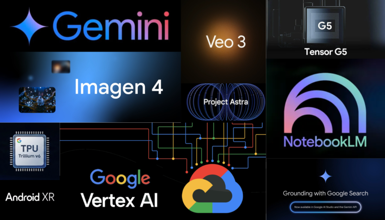
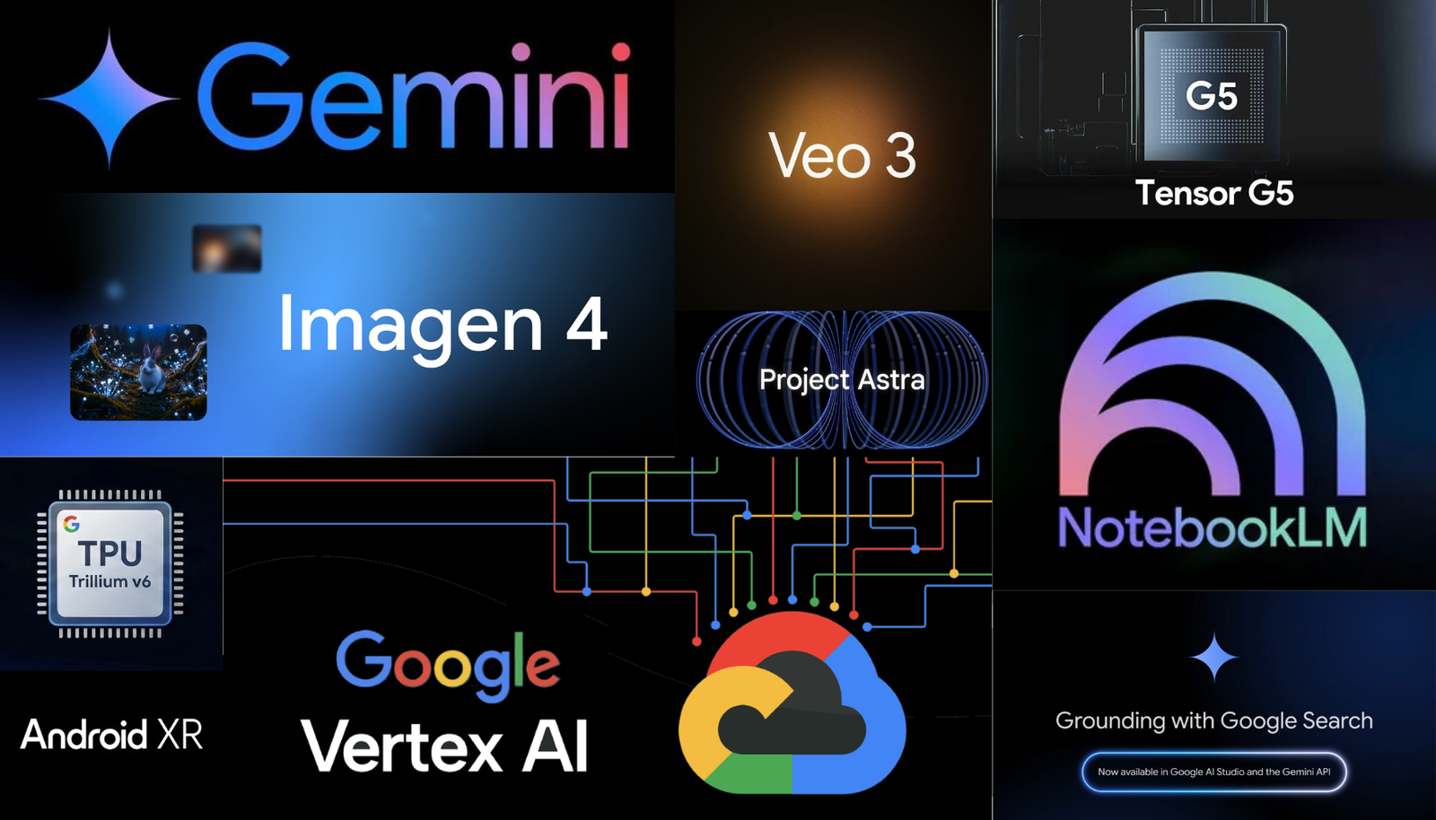
• Grounding with Google Search — Enterprise programs can use real-time web data to ground Gemini replies, which can cut down on hallucinations by up to 60%. That’s a statistic worth thinking about for a while. Every time, enterprise buyers ask about hallucination reduction first.
• Vertex AI Agent Builder — Companies build custom AI agents without writing code. Agents handle customer service, data analysis, and workflow automation.
• Imagen 4 — Google’s newest image creation model, and it makes product images that seem like actual photos. It helps e-commerce businesses make a lot of catalog photos, which saves them a lot of money on production.
• Veo 2 —Creating videos for marketing teams. Brands make product demos and posts for social media right from text prompts.

Also, Google Cloud’s Gemini Code Assist has revolutionized how developers work in ways I really didn’t expect to happen this quickly. The tool now writes about 35% of the new code that enterprise developers write on the platform. It works with more than 20 programming languages and connects directly to GitHub, GitLab, and Bitbucket. Fair warning: the learning curve is real, but once developers learn how to prompt it well, the productivity gains compound fast.

Enterprise case study: Wendy’s — Wendy’s is a fast-food business that uses Google Cloud’s GenAI to run its drive-through ordering system. The AI can have conversations like a person, suggest other menu choices, and make complicated changes. Wendy’s said that the average time it took to fill an order went down by 22 seconds at pilot locations. Because of this, the corporation added the technology to more than 1,000 places in 2026. Twenty-two seconds per automobile times thousands of places is a lot of arithmetic.

Enterprise case study: Mercedes-Benz — Mercedes-Benz employs Vertex AI to run its virtual assistant in cars. Drivers ask inquiries in everyday language about how to get about, how to set up their car, and services nearby. The system handles queries locally using bespoke TPU processors, which keeps latency low even when there is no cellular connection. That final aspect is important; no one wants their vehicle assistant to stutter because the signal is weak.

The table below shows how Google Cloud’s GenAI products stack up against those of its biggest competitors:

Feature	Google Cloud (Vertex AI)	AWS Bedrock	Microsoft Azure AI
Foundation models available	200+	150+	120+
Custom model training	Yes (TPU v6e)	Yes (Trainium)	Yes (GPU clusters)
Code assistance	Gemini Code Assist	Amazon Q Developer	GitHub Copilot
Image generation	Imagen 4	Titan Image	DALL-E 3
Video generation	Veo 2	Limited	Sora (preview)
Agent builder (no-code)	Yes	Yes	Yes (Copilot Studio)
On-device deployment	Yes (Gemini Nano)	Limited	Limited
Data residency controls	40+ regions	30+ regions	60+ regions

In 2026, Google’s price strategy for Vertex AI became significantly more competitive, which is important. The company started charging per-token prices that are about 20% lower than those of its competitors for workloads with a lot of tokens. who change has brought in mid-sized businesses who couldn’t afford the infrastructure expenditures before, which is a sensible land-and-expand move, not just kindness.

Hardware and On-Device GenAI: Pixel, TPU, and Android

Google added to its list of real-world GenAI 2026 hardware deployments with some really cool on-device features. The Pixel 9 series came out with Gemini Nano for processing on the device, but the Pixel 10, which came out in late 2025, goes far further. I’ve tried out a lot of products that say they have AI built in, and most of them don’t live up to their claims. This one really works.

Pixel 10 GenAI features that run only on the device:

• Live translation — Real-time conversation translation in 15 languages, no internet required.
• Smart photo editing — Object removal, background replacement, and lighting adjustment all powered by local AI processing.
• Call screening with context — The phone summarizes incoming calls, detects spam with 99.2% accuracy, and provides real-time transcription.
• Adaptive battery management — GenAI predicts app usage patterns and optimizes charging cycles. Google claims a 15% improvement in battery longevity over two years, which — if it holds up — is a meaningful quality-of-life win.

But the bigger story here is how Android is using GenAI in more ways. Android 16, which came out in the middle of 2026, has GenAI features at the system level that any compatible devices can use. In particular, any phone with 8GB or more of RAM may run a lighter version of Gemini Nano. That includes a lot of gadgets.

Google’s cloud-side GenAI architecture is powered by TPU v6e (Trillium) chips. For inference tasks, these bespoke processors are 4.7 times faster than TPU v5e. Google has put them in all of its key data center areas. Because of this, API response times for Gemini models have fallen by about 40% since early 2025. Faster replies aren’t just good to have; they’re the difference between a product that people actually use and one that makes them angry.

The Pixel 10’s Google Tensor G5 chip is also a real step forward for AI on devices. The chip’s neural processing unit takes up 30% more silicon space than the Tensor G4’s. This lets the Pixel 10 run Gemini Nano 2.0, which can do multiple tasks at once, including evaluating a photo while processing a voice command. People don’t know how important that kind of simultaneous processing is in everyday life.

For people who care about privacy, the on-device method is the most important. All processing happens on the device, so your photographs, conversations, and personal information never leave the device. And it’s a choice made on purpose, not just for technical reasons.

User Adoption Patterns and Performance Metrics

Knowing how people really use these tools explains why Google added so many real-world GenAI 2026 to its list. The patterns of adoption tell a really interesting narrative, and some of them startled me.

Search GenAI adoption:

• AI Overviews now appear in results across 200+ countries and territories
• Users aged 18–34 engage with AI Overviews 2.3 times more often than users over 55
• Mobile users interact with GenAI search features 40% more than desktop users
• Average session duration has increased by 12% since AI Overviews launched

Workspace GenAI adoption:

• Enterprise customers using Gemini in Workspace grew 300% year-over-year
• The most-used feature is email drafting in Gmail, followed by document summarization
• Small businesses (under 50 employees) show the highest per-user engagement rates
• Customer satisfaction scores for Workspace increased 8 points after GenAI integration

Cloud GenAI adoption:

• Vertex AI active customers surpassed 150,000 organizations in Q1 2026
• The average enterprise runs 3.7 GenAI models in production on Vertex AI
• API calls to Gemini models grew 500% between January 2025 and January 2026
• Healthcare and financial services are the fastest-growing verticals

Some areas, on the other hand, are taking longer to adopt. Because of compliance rules, government entities are still being careful. Google has gotten FedRAMP approval for a number of GenAI services, but it takes the public sector 12 to 18 months longer to buy things than the private sector. That gap isn’t going to close any time soon; it’s built in.

In addition, there is an interesting regional trend that is worth keeping an eye on. GenAI features are being adopted the fastest by businesses in North America and Europe. At the same time, adoption is picking up speed in Asia-Pacific regions, especially in Japan, South Korea, and India. Google has made Gemini models more relevant to these markets, which has improved the quality of responses in languages other than English.

Performance benchmarks that matter:

1. Gemini 2.5 Pro scores 92.1% on the MMLU benchmark — the highest of any commercial model as of mid-2026.
2. Gemini 2.5 Flash processes requests at 350 tokens per second, making it genuinely suitable for real-time applications.
3. Imagen 4 achieves a FID score of 2.1, indicating near-photorealistic image quality.
4. Gemini Code Assist acceptance rate sits at 38% — meaning developers accept more than one in three suggestions, which is actually impressive in practice.

These figures aren’t only for bragging rights. Models that are faster give quicker answers, models that are more accurate need fewer changes, and models that are better at making images cut down on manual design effort. Google’s AI research blog is a great place to find many of these benchmarks. That kind of openness, even if it’s not perfect, helps businesses make better judgments about where to deploy, and I’d like to see more competitors follow suit.

What’s Next: Google’s GenAI Roadmap for Late 2026

The speed at which Google added real-world GenAI 2026 deployments to its list strongly suggests that it has even bigger ambitions in the works. There are a lot of signs that show what’s coming, and the roadmap is something to pay attention to right now.

Project Astra is Google’s plan to make a universal AI assistant that can see, speak, and act all at the same time. Early tests suggest that an AI can see through your phone’s camera, grasp the situation, and do things in other apps. By the end of 2026, there should be a small public preview. I’ve seen the demo video more than once. It looks like science fiction until you understand that the parts are already on their way.

It looks like Google is testing the Gemini Ultra 2.0, which is their most powerful model. It was made for complicated scientific reasoning, analyzing large documents, and working with multiple agents. Enterprise clients that are part of Google’s Trusted Tester program are already testing it. This is the model tier that might really give frontier competitors a run for their money in research-grade applications.

Android XR is Google’s platform for extended reality. It employs GenAI to make experiences that are immersive and aware of their surroundings. In 2025, Samsung released the Project Moohan headgear, which runs on Android XR. Also, additional hardware partners are likely to unveil devices that use this platform. Because of this, the ecosystem could grow faster than most people think.

More options for other industries: Google Cloud is making ready-made GenAI solutions for healthcare, retail, manufacturing, and education. These aren’t just regular tools with a new name. They’re taught on data from their own field and made to follow regulations that are specific to that field, like HIPAA for healthcare. In businesses that are regulated, that level of detail is quite important.

So what does this mean for businesses and developers? The time for trying new things is really running out. GenAI is now fully in production, and organizations that haven’t started using these technologies yet risk slipping behind competitors who have, sometimes by more than a year.

Conclusion

Google expanded its list of real-world GenAI 2026 deployments across every major product category. Search, Workspace, Cloud, and hardware all received substantial, production-ready AI features. And importantly, these aren’t experimental toys — they’re tools that billions of people and hundreds of thousands of organizations rely on daily.

The numbers speak clearly. Two billion monthly users interact with AI Overviews. Over 150,000 organizations run GenAI on Vertex AI. Pixel devices process AI tasks locally without sending data to the cloud. Enterprise adoption, moreover, continues accelerating across industries — with no obvious sign of slowing down.

Your actionable next steps:

1. Audit your current tools — Check whether your Google Workspace or Cloud subscriptions include GenAI features you’re not already using. You might be paying for them.
2. Start with one workflow — Pick a single repetitive task and test whether Gemini can handle it. Email drafting and document summarization are easy wins with low stakes.
3. Evaluate Vertex AI — If you’re building customer-facing applications, explore Vertex AI’s agent builder and grounding features before assuming you need to build from scratch.
4. Monitor the roadmap — Follow Google’s AI blog for updates on Project Astra and Gemini Ultra 2.0. Both could shift what’s possible in your stack.
5. Train your team — GenAI tools only deliver value when people know how to use them well. That part’s on you, not the technology.

The main point of the Google expanded list real-world GenAI 2026 tale is that it is about practical AI that operates on a large scale. Google has shown that it can send GenAI well past the demo stage. It’s now up to businesses and users to use it. Waiting is no longer a neutral choice.

FAQ

The subject of how EV charging robot automation technology works is no longer simply an academic one. These devices are coming into parking garages and fleet depots right now, plugging in automobiles without anyone having to touch a cable.

And to be honest? When you think about it, that’s crazy.

Autonomous charging robots are a real change in the infrastructure for electric vehicles. The charger comes to the drivers instead of them looking for open ones. Also, this technology solves genuine problems, such making it easier for disabled drivers to get around, charging fleets overnight, and making the most of parking spaces. I’ve been following this space for years, and the speed at which businesses are using it has even astonished me.

But how could a robot really discover the charging port on your car, line itself up properly, and plug it in? The answer has to do with sensor fusion, precise actuators, and some very smart software. Here’s a list of all the layers.

How EV Charging Robot Automation Technology Works at the Hardware Level

To understand how EV charging robot automation technology works, you need to know how the machine itself works. Most designs have the same basic structure, but how they are made might be very different from one manufacturer to the next.

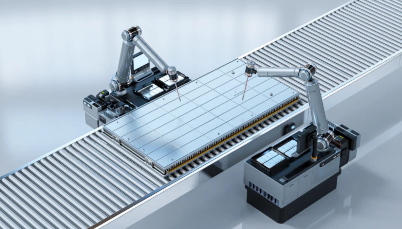
The mobile base is basically an autonomous mobile robot (AMR). It moves through parking structures on wheels or tracks. Companies like Volkswagen showed off early prototypes with rolling units that had batteries. In the meantime, companies like EV Safe Charge and Evar have released commercial versions. I’ve seen video of the VW prototype driving through a garage, and it does so with an almost alarming amount of confidence.x

The mobile base has a robotic arm on top of it that can usually move in six different ways. That means it can reach, twist, and angle the connector into almost any position on the charge port. In particular, these arms are very similar to industrial robots, which are the same kind of robots that work on factory assembly lines. When you see the arm in action up close, be warned: the pace is slower than you may think, but the precision is astounding.

The connector end-effector is the part that does the work. It has a standard CCS, CHAdeMO, or Type 2 plug, and some models employ a universal adaptor system. The gripper must exert the right amount of force—enough to hold the connector in place but not so much that it breaks the port. It sounds easy to make that balance, but it’s not.

Some important hardware parts are:

• LiDAR sensors for navigation and obstacle detection
• Depth cameras (often Intel RealSense or similar) for close-range alignment
• Force-torque sensors at the wrist joint for safe plug insertion
• Onboard battery pack to power the robot between docking stations
• Wireless communication module for fleet management integration

The hardware by itself isn’t that great. The software that controls the EV charging robot is what makes it really operate, and that’s where things get fascinating.

Sensor Fusion and Positioning: The Brain Behind Autonomous Docking

This is where the technology for automating EV charging robots gets interesting. A robot can’t just pull up and assume where the charge port is; it needs to be accurate to within a millimeter. So, these systems need different kinds of sensors to work together. It’s like the robot is using its eyes, hands, and memory all at once.

Simultaneous Localization and Mapping (SLAM) takes care of the large picture. The robot keeps track of where it is in the parking complex while making a map of it. Many teams use ROS (Robot Operating System) as a base for their SLAM programs. The robot knows where it is in relation to walls, columns, and parking slots. This is a lot harder to do in a concrete garage than it sounds because GPS doesn’t work well in certain places.

Computer vision takes care of figuring out what kind of vehicle it is. Cameras can tell the make, model, and direction of a car, while neural networks trained on thousands of pictures of cars can find the exact location of the charge outlet. Some systems also examine license plates to find the right billing request for a car. When I first looked at the specs, I was amazed to see that the plate-reading part works for both authentication and navigation.

During the last approach, close-range depth sensing takes over. Cameras that use structured light or time-of-flight produce a 3D point cloud of the region around the charge port. The robot’s software then compares this point cloud to known port shapes. In particular, it figures out the exact depth, angle, and position needed for insertion. We mean accuracy of less than 5mm.

The last layer is force feedback. Force-torque sensors pick up on resistance patterns when a plug is inserted. Too much force from the side? The arm moves. The connector clicks into place, and the robot says that docking was successful. This is like how you would feel the plug pop into place by hand, but it’s doing it without seeing it, using only sensor data.

The sensor fusion pipeline usually goes like this:

1. Receive charging request with vehicle location data
2. Move to the general parking area using SLAM
3. Identify the target vehicle with computer vision
4. Approach and localize the charge port with depth cameras
5. Execute the docking motion with force-guided insertion
6. Verify electrical connection and begin charging
7. Monitor the session and undock when complete

But in the actual world, this is harder than it sounds. In parking garages, the lights change all the time and cars park at strange angles. Charge ports might be hidden by snow, debris, or aftermarket parts. So, reliable EV charging robot automation technology needs to be able to handle edge circumstances well, and edge cases are where most systems still have problems.

Real-World Deployment Challenges and How Manufacturers Solve Them

It’s one thing to know how EV charging robot automation technology works in a lab. Putting it in a crowded parking garage is a whole different story.

I’ve talked to engineers at two different robots companies about this, and the problems they talk about are worse than what you see in product demos.

Parking variability is the biggest headache. Drivers park crooked, too close to walls, or across lines instead of neatly in the middle. So, the robot needs a lot of reach and the ability to change its approach. Some systems fix this by making drivers park in painted guiding zones, while others just make their algorithms more flexible. The guide zone method works, but getting drivers to actually use it is a whole other issue.

Connector standardization remains a genuine obstacle. North America is moving toward the NACS (North American Charging Standard) because Tesla’s connector has become the SAE J3400 standard. Older cars, on the other hand, still use CCS1. Robots need to have more than one connector or employ adapter mechanisms, which makes them more complicated and more likely to break.

Safety certification is very important and not up for debate. These robots work near people and must follow ISO 10218 for industrial robot safety and new rules for collaborative robotics. They also have to deal with things that come up out of nowhere, like a youngster racing by or a shopping cart rolling into their path. You have to have emergency stop systems and collision-avoidance protocols. They’re the whole game.

Power management makes things difficult because they depend on each other. The robot relies on batteries and needs enough power to move, dock, and maybe even transfer electricity. Some designs come with their own battery packs that send power to cars. Some people connect a mobile cable management system to fixed electricity lines. The battery-carrying method slows down charging speed, but it lets you charge anywhere, usually up to 22 kW, which is fine for overnight charging but not enough for a quick lunchtime top-up.

Communication protocols tie everything together. The robot needs to be able to talk to the car, the building management system, and the cloud platform. OCPP (Open Charge Point Protocol), is what lets chargers talk to the network. ISO 15118 also lets the car and charger authenticate each other when they are plugged in. The robot acts as a mobile OCPP-compliant charge point. It’s a surprisingly well-designed piece of protocol.

This is how the main methods stack up:

Feature	Battery-Carrying Robot	Cable-Tethered Robot	Fixed Robotic Arm
Mobility	Fully mobile	Limited range	Stationary
Charging speed	Slower (typically 7–22 kW)	Fast (up to 150 kW+)	Fast (up to 300 kW+)
Infrastructure cost	Lower initial cost	Moderate	Higher initial cost
Vehicles served per unit	Multiple, sequentially	Multiple within range	One at a time
Best use case	Fleet depots, airports	Parking garages	Dedicated charging hubs
Navigation complexity	High	Medium	Low
Example	VW mobile charger concept	Evar robot	Rocsys automated connector

Each method has its own pros and cons when it comes to EV charging robot automation technology, and the best one for you will depend on where you plan to use it. There isn’t a clear winner here, but sellers won’t always tell you that.

The Software Stack: AI, Path Planning, and Fleet Orchestration

There are many layers to the software that runs the equipment that automates EV charging robots. This is the section that really sets the serious gamers apart from the demo-ware.

Perception software turns raw sensor data into valuable information. Convolutional neural networks (CNNs) can find objects like cars, charge ports, people, and other things that get in the way. These models learn from big amounts of parking data. They also need to execute in real time on edge computing hardware that is built into the robot. NVIDIA Jetson modules are a common choice for this kind of work. The real test is whether these models will perform well at 2am in a dark garage, not just when everything is perfect.

Path planning algorithms tell the robot where to go. A* and RRT (Rapidly-exploring Random Trees) algorithms find pathways that don’t hit anything in crowded parking lots. The planner keeps getting better as more sensor data comes in. In particular, the robot changes its route several times each second to avoid things that are in its way. A lot of math is going on behind the scenes while the robot moves toward your Tesla.

Motion control software turns planned pathways into commands for motors. PID controllers and more powerful model predictive control (MPC) algorithms make sure that movement is smooth and accurate. The robotic arm employs inverse kinematics to figure out the exact angles of the joints needed to move the connector to the right place. This math runs a lot of times every second. (And yes, it really is as cool as it sounds.)

Fleet orchestration controls many robots in a building. The orchestration layer takes care of:

• Task assignment — which robot charges which vehicle
• Queue management — prioritizing vehicles by departure time or state of charge
• Traffic coordination — preventing robots from colliding with each other
• Energy optimization — scheduling charging sessions to cut peak demand costs
• Predictive maintenance — flagging robots that need servicing before they fail

In the same way, the cloud platform lets you monitor and analyze things from afar. Dashboards let facility managers keep track of how often robots are used, how much energy they use, and how many times they charge. Amazon Web Services and other similar platforms often provide as the backbone for these systems’ IoT. It’s basically a logistics platform that also connects cars.

Machine learning improves performance over time. Every time you try to dock, it makes data. Successful connections make good approach tactics stronger, whereas failed attempts lead to analysis and model retraining. So, the longer robots work, the better they get at dealing with tough situations. This loop of constant development is at the heart of how EV charging robot automation technology grows in real life. It’s also why first-mover deployments, even if they’re not perfect, are so important in terms of competition.

The Business Case: Why Autonomous Charging Makes Financial Sense

Look, it’s important to know how EV charging robot automation technology works since the economics are really interesting. There’s a real bottom line reason for this technology, not just because it’s cool.

The main value proposition is based on space efficiency. Traditional charging stations need parking spaces that are set aside for them and have stationary equipment. One charging robot can move between cars and serve 8 to 12 parking slots. So, people that run parking garages don’t give up areas that may make money to put in chargers. In a garage in the city that charges $40 per place per day, such math adds up quickly.

Lower installation costs are quite important. It costs between $15,000 and $50,000 to run high-voltage wiring through a concrete parking structure for each recharge station. Robots don’t need as many fixed power drops, and a single power station may power a whole floor with mobile robots. Also, it is much easier to add features to existing buildings, since most parking structures in the U.S. are already built.

Over time, savings on labor add up. Fleet operators now pay people to plug in cars overnight, but self-driving robots would eliminate this cost completely. Also, they work around the clock without breaks, overtime, or having to deal with scheduling problems. Fleet managers I’ve talked to say that for mid-sized EV fleets, they spend between $80,000 and $120,000 a year only on charging labor.

Accessibility compliance is useful for following the rules. The Americans with Disabilities Act says that charging stations must be easy to get to. Because robots come to the car, they make it easier for people with disabilities to operate the car by design. The driver never has to deal with heavy cables or move charging equipment around. From a compliance point of view, that’s a no-brainer.

Grid optimization makes things better for utilities. Smart orchestration software can move charging loads to times when they are less busy. Charging automobiles one at a time instead of all at once lowers peak demand charges. As a result, the people that run the facilities pay less for electricity. The U.S. Department of Energy says that managed charging is important for keeping the grid stable. Interestingly, robotic systems are better at managed charging than fixed chargers with people who are impatient.

The total cost of ownership assessment is becoming more and more in favor of robotic solutions for facilities with more than 50 electric vehicles. Even while the cost of a robot up front is still significant (usually between $50,000 and $150,000), the savings on infrastructure and the increased efficiency of operations mean that the robots pay for themselves in 3 to 5 years in places where they are used a lot. Be warned: the payback window is based on high utilization rates. A garage that is just half full changes the math a lot.

Conclusion

How EV charging robot automation technology works is a well-planned combination of hardware, sensors, AI, and fleet software. These devices use LiDAR navigation, computer vision, force-guided docking, and intelligent orchestration to charge themselves reliably. I think the software stack is the more amazing feat, not the hardware.

The technology is genuine and in use right now. It is getting better quickly thanks to machine learning and lower costs for parts. As more people buy electric vehicles and parking companies hunt for better ways to charge them, the business argument gets stronger. The unit economics are getting better.

If you’re looking into EV charging robot automation technologies, here are some things you can do next:

• For facility managers: Request pilot proposals from vendors like Rocsys, Evar, or EV Safe Charge. Start with a small deployment to test performance in your specific environment.
• For fleet operators: Calculate your current per-vehicle charging labor costs. Compare against robotic solutions for overnight depot charging.
• For technology professionals: Explore the ROS ecosystem and OCPP standards. The intersection of robotics and EV charging offers growing career opportunities.
• For investors: Watch for companies achieving consistent sub-30-second docking times. That’s the threshold where EV charging robot automation technology becomes truly competitive with human-operated charging.

There won’t be an autonomous charging transition. It’s already here, and knowing how it works will help you make better choices regarding infrastructure, investment, and adoption.

FAQ

References

• Editorial photograph for «How EV Charging Robot Automation Technology Actually Works».
• Volkswagen
• ROS (Robot Operating System)
• NACS (North American Charging Standard)
• ISO 10218
• OCPP (Open Charge Point Protocol)
• Amazon Web Services
• The U.S. Department of Energy

Dynamic batching for encoder-decoder MT training & generation is one of the most powerful optimizations you can perform for machine translation workloads. If you are using encoder-decoder models such as mBART, T5 or MarianMT, you presumably have already seen the problem. Fixed-size batches waste a lot of GPU RAM on padding tokens, and that waste adds up quickly.

As a result, throughput falls. Latency spikes Your cloud bill climbs faster than your model’s BLEU score I’ve spent years refining MT pipelines and this one adjustment always makes more of a difference than other architectural tweaks. This book will cover practical strategies on how to setup dynamic batching in encoder-decoder architectures, handle variable length inputs, increase GPU utilization and reduce inference latency in production.

If you are training or providing a translation model at scale, these techniques will help you squeeze every last FLOP out of your hardware.

Why Encoder-Decoder Models Need Dynamic Batching

Encoder-decoders process two sequences of varying length: a source sequence and a target sequence. That’s a special problem most people overlook.

Unlike decoder-only models (GPT type), you are dealing with two padding dimensions at once. That’s more than twice the waste from naive fixed batching – and it accumulates at every attention layer.

Say , for instance , you have a batch where one source sentence is length 5 and another is length 120. In static batching, every sequence is padded to 120 tokens. That little statement now adds 115 meaningless padding tokens to every single attention computation. Multiply that across thousands of training samples and you’re burning major compute for practically nothing.

This is solved by dynamic batching for encoder-decoder MT training and generation, which batches sequences of similar lengths. This results in considerably less padding, greater memory use and faster wall-clock training times. Furthermore, this method applies to all main encoder-decoder frameworks, so you are not bound to a single tool.

But here is why it’s extremely critical for MT workloads specifically:

• Source and target lengths are correlated but not identical. German sentences are generally longer than English sentences. Tokenizing sentences with SentencePiece makes the Chinese sentences shorter. You can’t just optimize one side.
• Batch composition directly affects gradient quality. Poorly batched training data can induce subtle biases towards specific length distributions, and it’s surprisingly hard to diagnose.
• Autoregressive decoding is sequential. The time to finish a batch during generation is determined by the slowest sequence in a batch. One long outlier takes everyone hostage.

These effects are particularly important for models such as mBART and T5. Their cross attention layers take both encoder and decoder representations, such that padding waste compounds at every layer, not just once.

Core Techniques for Dynamic Batching in MT Workloads

There are several proven ways for building dynamic batching for encoder-decoder MT training & generating pipelines. They are all a real trade-off of complexity vs. performance — I’ll give you the honest version of each.

1. Length-based bucket batching

This is the most typical strategy and honestly a wonderful place to start. You arrange your dataset by source length, bucket examples of comparable size and make batches of max token size instead of max example size.

Instead of always batching up 32 instances, you might batch up 64 short statements, or 8 long ones. The important parameter is total tokens per batch, not examples per batch. Fairseq has a native implementation of this using the --max-tokens flag, which is one of the cleanest implementations I’ve seen.

2. Token-budget batching

Token-budget batching also limits the maximum number of tokens each batch. The data loader continues to add examples until adding the next one would exceed the budget. This naturally results in bigger batches for short sequences and smaller batches for long sequences.

Here is a simple implementation pattern:

def token_budget_batcher(sorted_examples, max_tokens=4096):
    batch = []
    current_tokens = 0

    for example in sorted_examples:
        src_len = len(example["source"])
        tgt_len = len(example["target"])
        max_len = max(src_len, tgt_len)

        needed = max_len * (len(batch) + 1)

        if needed > max_tokens and batch:
            yield batch
            batch = []
            current_tokens = 0

        batch.append(example)

    if batch:
        yield batch

Fair warning: the token budget you specify here directly correlates with your GPU RAM ceiling, so start small.

3. Multi-dimensional sorting

Sorting just by source length is suboptimal for encoder-decoder models. Order by source length and goal length. This is difficult to set up, but it cuts the padding on both sides of the model at the same time. The OpenNMT data loading configuration enables this. The padding reduction is much better than single axis sorting.

4. Dynamic padding with attention masks

Instead of padding to a global maximum you pad to the largest sequence in each batch. Low complexity, real gains This is the smallest possible optimization combined with adequate attention masking Specifically, Hugging Face Transformers provides DataCollatorForSeq2Seq for this purpose. If you’re already in that ecosystem, this is a no-brainer launching point.

Technique	Padding Reduction	Implementation Complexity	Training Stability
Fixed batching (baseline)	None	Low	High
Length-based bucket batching	40-60%	Medium	High
Token-budget batching	50-70%	Medium	Medium
Multi-dimensional sorting	60-80%	High	Medium
Dynamic padding + attention masks	20-40%	Low	High

Memory Trade-Offs and Throughput Optimization

It is important to understand memory behavior for dynamic batching for encoder-decoder MT training & generating systems. GPU memory is not infinite and dynamic batching creates variability which can lead to out of memory (OOM) issues if you are not careful – and you will be, the first time you push it too far.

Peak memory usage depends on batch size. Static batching is deterministic in memory. Dynamic batching can use substantially more memory with a batch of long sequences than with a batch of short sequences. You need headroom. Begin with a cautious token budget and increase it incrementally while keeping an eye on peak allocation.

Gradient accumulation makes things more smooth. As the batch sizes vary, gradient accumulation aids in maintaining consistent effective batch sizes. Accumulate gradients across numerous dynamic batches before weight update. This keeps training stable and GPU utilization high – the combo that actually works in practice.

And some practical tips about optimization:

• Profile before optimizing. Determine if you are memory-bound or compute-bound with PyTorch Profiler. Each scenario has a somewhat different fix and guessing poorly loses time.
• Pre-sort your data once. Don’t re-sort each epoch. Sort by length, shuffle within length buckets so that it stays random but doesn’t lose efficiency.
• Monitor padding ratios. Track the % of padding tokens of each batch. This is kept under 10% with healthy dynamic batching. If you’re seeing 20%+ you need to work on your bucket approach.
• Use mixed precision training. FP16 or BF16 halves memory usage per token, thereby doubling your token budget while altering nothing else.

But the main story is the throughput benchmarks. In reality, replacing fixed batching with token-budget dynamic batching usually results in 1.5x to 3x throughput gains for encoder-decoder MT models. The gains are highest when your dataset has high length variance – language pairs like English-German or English-Chinese profit enormously. I was shocked when I first measured it accurately; the disparity is larger than the theory predicts.

Memory efficiency is also improved by 30-60% in most systems. This implies you can train with larger effective batch sizes, or with smaller GPUs for the same workload – both of which have actual cost considerations.

Keep an eye on gradient noise. Dynamic batching modifies the mix of mini-batches. Batches with predominantly short sequences have more examples and hence higher gradient signal. There is less data for batches with long sequences. As a result, the gradient variance grows throughout training. Learning rate warmup and gradient cutting help to mitigate this. Don’t skip these.

Dynamic Batching for Inference and Generation

Training is just the beginning. Dynamic batching for encoder-decoder MT training & generation is also very important in inference time. And honestly the latency impact is more typically seen during serving than training.

The tail-latency problem is genuine. Autoregressive decoding generates tokens one-by-one for each sequence in a batch . The batch will not be returned until the longest output sequence is complete. One very long translation can block the whole batch — and in production that directly translates into spikes in user-facing delay.

There are a couple of techniques that address this:

• Early stopping per sequence. If a sequence generates an end-of-sequence token, remove it from active computation, and fill its slot with a new request. This is frequently termed continuous batching or iteration-level scheduling – and it’s one of the most powerful serving optimizations you can do.
• Request queuing with timeout. Queue incoming requests for a short duration, batch inputs of similar length and then send to the model. Set a maximum wait time to keep latency in check; 20-50ms is a reasonable starting value for most MT applications.
• Speculative length prediction. Predict output length with a lightweight model and route requests to batches based on that. This is surprisingly effective for MT, where output length is meaningfully correlated with input length.

Importantly, serving frameworks like Triton Inference Server support dynamic batching natively. You configure a maximum batch size and a batching window, and the server automatically groups requests that arrive within that window. It’s worth the setup time.

If you are using encoder-decoder models in particular, you need also consider:

• Encoder output caching: Run the encoder once and reuse the representations for all decoding processes. This is normal procedure . But if the composition of the batch changes mid-sequence , dynamic batching can make the cache management tricky .
• Batch in separate encoder/decoder: The encoder processing is trivially parallel. Decoder processing is sequentially. Their throughput profiles are very different thus you can also batch encoder passes aggressively while keeping decoder batches smaller.
• KV-cache handling: Each active sequence has a key/value cache that grows with the length of the output. Dynamic batching must be aware of this expanding memory footprint. Otherwise you would get OOM problems mid-generation.

But the point is, your decisions should be driven by production latency requirements. If you want real-time MT (less 200ms), you will want small batches with strict timeouts. Use big token budgets and extended batching windows to maximize throughput for large translation workloads. But the strategies above provide you the knobs to tweak for any scenario—you’re not stuck with one strategy.

Implementation Patterns for Popular Frameworks

Your implementation of dynamic batching for encoder-decoder MT training & generation will depend on your framework. These are real patterns for the most frequent tools. The ones I personally use.

Hugging Face Transformers and Datasets

The DataCollatorForSeq2Seq handles dynamic padding automatically. Combine it with a Sampler that groups by length:

from transformers import DataCollatorForSeq2Seq

collator = DataCollatorForSeq2Seq(
    tokenizer=tokenizer,
    model=model,
    padding=True, # Dynamic padding to batch max
    max_length=None, # No global max
    pad_to_multiple_of=8 # Tensor core alignment
)

Setting pad_to_multiple_of=8 is a little but crucial detail – it aligns tensor dimensions to multiples of 8, which improves performance on NVIDA Tensor Cores. Easy to overlook, simple victory.

Fairseq

Fairseq’s data loading is built around dynamic batching from the ground up. Use --max-tokens instead of --batch-size:

fairseq-train data-bin/wmt14_en_de \
    --max-tokens 4096 \
    --arch transformer \
    --required-batch-size-multiple 8

The --required-batch-size-multiple flag ensures batch sizes align for optimal GPU use. Moreover, Fairseq supports combining --batch-size with --max-tokens for a hybrid approach where both constraints apply at once — useful when you want a ceiling on both dimensions.

Custom PyTorch implementation

For full control, set up a custom BatchSampler:

1. Sort your dataset indices by source sequence length
2. Group indices into chunks where the total token count stays under your budget
3. Optionally shuffle the order of chunks (not within chunks) each epoch
4. Yield each chunk as a batch

That means this strategy is the most flexible. You can use target lengths, domain information, or language pair metadata in your batching logic – anything that pre-built solutions don’t offer. I’ve tried dozens of combinations this way, and that granular control is a lifesaver when your data is messy or domain-mixed.

ONNX Runtime for optimized inference

Export your encoder-decoder model to ONNX format for production use. ONNX Runtime supports dynamic axes, thus input form can vary from batch to batch. This naturally pairs with dynamic batching at the serving layer — and the benefits in inference speed are very astounding on optimal hardware.

Conclusion

Dynamic batching for encoder-decoder MT training & generation is not an option for heavy MT workloads; it is necessary infrastructure. Token-budget batching, multi-dimensional sorting, continuous batching for inference, and framework-specific implementations are some of the methods that can greatly improve the efficiency of your pipeline. Just by getting this correctly, I’ve seen teams slash their computing expenditures in half.

Begin with the easiest tasks. Change from fixed batch sizes to token-budget batching. You can apply dynamic padding with DataCollatorForSeq2Seq or Fairseq’s --max-tokens. Keep an eye on your padding ratio and how much you use your GPU. Then, if your needs expand, start using more complex methods like continuous batching.

Here are the steps you need to take right away:

1. Find out what your current padding ratio is. If it’s higher than 15%, you have a lot of space to improve, and the solution is simple.
2. This week, set up token-budget batching in your training loop. The code really isn’t that hard.
3. Keep track of memory use across batches to identify the best token budget for you without causing OOM problems.
4. Depending on your architecture, you should look at using Triton or a custom solution for serving-side dynamic batching.
5. Keep track of throughput in tokens per second, not examples per second. That’s the number that really matters for dynamic batching for encoder-decoder MT training  & generation pipelines; everything else is just a proxy.

What does it all mean? Less wasted computing power, faster training, less lag, and smaller cloud fees. Static batching isn’t good enough for your encoder-decoder MT models.

FAQ

References

• Editorial photograph for «Dynamic Batching for Encoder-Decoder MT Training & Generation».
• mBART
• T5
• Fairseq
• OpenNMT
• Hugging Face Transformers
• PyTorch Profiler
• Triton Inference Server
• ONNX Runtime

Most teams don’t realize how important it is to select the appropriate version control tool until it’s too late. A comprehensive comparison of software configuration management systems in 2026 reveals some genuinely unexpected distinctions between the leading candidates. Fossil, Git, and Mercurial all have unique advantages, but despite what you’ve heard about Git’s supremacy, that’s not the whole picture.

The majority of teams simply take Git and go. And really? That’s okay sometimes. However, two years later, you will be fighting your own workflow if you choose a tool without considering the trade-offs.

In order to help you determine which system best suits your team’s requirements, this guide breaks down features, performance, workflows, and real-world use cases. In addition, we’ll go over setup procedures so you can do these things rather than just read about them.

Why a Software Configuration Management Systems Comparison 2026 Still Matters

Monitoring code changes is only one aspect of version control. Because it is the foundation of contemporary software development, choosing the incorrect tool causes friction that gradually increases over time.

Git dominates market share. That cannot be disputed. However, not every team is a good fit for dominance. I’ve seen small startups drown in Git complexity when, for a fraction of the setup cost, Fossil would have been a perfect fit. A flawless interactive rebase on a shared branch took three days to unravel for a five-person agency I consulted for; this scenario could not have occurred in the same manner under Fossil’s model.

A comparison of software configuration management systems is particularly pertinent at this time due to several factors:

• AI-assisted development generates more code changes, increasing repository stress
• Remote-first teams need tools that handle distributed workflows gracefully
• Compliance requirements demand better audit trails and traceability
• Monorepo adoption is growing, pushing tools to their scalability limits
• Supply chain security makes provenance tracking a genuine priority — not just a checkbox

In addition, things have actually changed. In 2020, Mercurial lost its Bitbucket residence. Users who are sick of piecing together five different tools have quietly embraced Fossil. Git continues to develop with partial clones and sparse checkouts. As a result, presumptions made even two years ago might no longer be valid; I’ve had to change my own thoughts on this several occasions.

An accurate comparison of software configuration management systems in 2026 must assess these tools based on their present capabilities. not a reputation. Not inertia.

Feature-by-Feature Comparison: Fossil vs Git vs Mercurial

Each tool’s fundamental characteristics disclose its design philosophies. In particular, they differ greatly in terms of branching models, integrated tools, and data storage.

Feature	Git	Mercurial	Fossil
Distributed VCS	Yes	Yes	Yes
Built-in wiki	No	No	Yes
Built-in bug tracker	No	No	Yes
Built-in web UI	Basic (gitweb)	Basic (hgweb)	Full-featured
Branching model	Lightweight branches	Named branches + bookmarks	Named branches (permanent)
Learning curve	Steep	Moderate	Gentle
Binary file handling	Poor (needs LFS)	Better	Good
Repository size limit	Scales well with workarounds	Moderate	Best for small-to-medium
Hosting options	GitHub, GitLab, Bitbucket	Heptapod, self-hosted	Built-in server
License	GPL v2	GPL v2	BSD
Single-file repository	No (.git directory)	No (.hg directory)	Yes (SQLite)
Autosync	No	No	Yes (optional)

This table illustrates the key finding of any comparison of software configuration management systems in 2026: Fossil offers the most integrated experience right out of the box, but Git wins on ecosystem breadth. This difference is greater than most people realize.

Git’s vast ecosystem is one of its main advantages. More than 200 million repositories are hosted on GitHub alone. There is no comparison in terms of extensions, integrations, and community support. Furthermore, Git’s lightweight branching enables sophisticated workflows in ways that other tools fall short. However, lightweight branches also cause teams to have 300 outdated remote branches with no obvious owner—a significant maintenance burden that is rarely acknowledged.

Behavioral consistency is one of Mercurial’s strong points; commands follow your expectations. That may seem simple until you’ve spent an afternoon troubleshooting a botched Git rebase. Its binary file handling outperforms Git without requiring any additional configuration, and the learning curve is noticeably softer. For instance, a design team that stores layered PSDs with code will notice the difference right away.

The advantages of Fossil is unique. A wiki, bug tracker, forum, and web server are all combined into one executable. It’s important to note that the entire repository is contained in a single SQLite database file; backup simply means “copy the file.” When I first set it up, I was taken aback by this. I continued to watch for the catch. That backup story alone makes the switch worthwhile for a lone consultant overseeing a dozen small client projects.

Setup Guides and Workflow Examples

Each tool requires significantly different amounts of effort to get started. For a software configuration management systems comparison 2026 that is genuinely useful rather than merely theoretical, here’s how to set them up and use each one.

Setting up Git:

1. Install Git from git-scm.com
2. Run git config --global user.name "Your Name"
3. Run git config --global user.email "you@example.com"
4. Create a repo with git init my-project
5. Add files with git add . and commit with git commit -m "Initial commit"

Git’s typical workflow runs on feature branches — you branch, make changes, then open a pull request. Although this scales beautifully for large teams, it adds real overhead for solo developers. Fair warning: the staging area alone confuses people for weeks. A common stumbling block is accidentally committing only part of a file’s changes because git add -p was run without fully understanding what it does — then spending 30 minutes figuring out why the build is broken on the remote but not locally.

Setting up Mercurial:

1. Install from mercurial-scm.org
2. Edit ~/.hgrc to set your username
3. Run hg init my-project
4. Add files with hg add and commit with hg commit -m "Initial commit"

Mercurial’s workflow feels more linear — and consequently, teams that care about clean, readable history often land here and stay. Bookmarks act as lightweight branches; named branches are permanent and show up in history. That permanence is either a feature or a bug depending on how you work. If your team treats branch names as meaningful documentation of intent, you’ll appreciate it. If you branch freely and experimentally, it can feel cluttered over time.

Setting up Fossil:

1. Download the single binary from fossil-scm.org
2. Run fossil init my-project.fossil
3. Run fossil open my-project.fossil
4. Add files with fossil add . and commit with fossil commit -m "Initial commit"
5. Launch the web UI with fossil ui

I’ve tested dozens of version control setups over the years, and Fossil’s onboarding is genuinely the smoothest. Five commands and you’ve got version control plus a bug tracker plus a wiki running locally. The autosync feature pushes every commit to the remote automatically. This prevents divergent histories. Therefore, it’s a near-perfect fit for small teams that want simplicity over flexibility. One practical tip: run fossil settings autosync on explicitly after opening a repository so you don’t have to remember to push — it’s not always the default depending on how the repo was initialized.

A real-world workflow comparison:

• Solo developer building a side project? Fossil’s all-in-one approach saves real time — no separate issue tracker, no separate wiki to configure. You can file a bug ticket, link it to a commit, and document the fix in the wiki without ever leaving the tool.
• Open-source project seeking contributors? Git on GitHub is the clear winner. The contributor pool is massive, and that’s not changing anytime soon.
• Enterprise team with strict compliance needs? Fossil’s immutable history and built-in audit trail deserve serious consideration. Alternatively, Git with signed commits works too, though it requires more setup discipline and consistent enforcement across the team.
• Data science team handling large binary files? Mercurial handles those more gracefully than vanilla Git — notably without needing LFS bolted on. A team storing trained model checkpoints alongside notebooks will notice the difference immediately.

Performance, Scalability, and Ecosystem in 2026

As soon as your repository expands beyond the scope of a hobby project, performance becomes important. This section of our comparison of software configuration management systems for 2026 looks at how each tool truly manages scale, not just what the marketing claims.

For large codebases, Git performance exceptionally well. Git’s ability to manage extremely large repositories was demonstrated by Microsoft’s migration of the entire Windows codebase. This is made possible by features like Git’s virtual filesystem, sparse checkout, and partial clone. But without Git LFS, Git has a terrible time handling big binary files. Furthermore, initial cloning can be excruciatingly slow due to very long histories. I’ve seen developers put off cloning a repository for more than twenty minutes. That isn’t speculative. For CI environments where full history is not required, one useful mitigation is to use git clone --depth 1; on large repositories, this can reduce clone times from minutes to seconds.

For the majority of workloads, Mercurial’s performance is comparable to Git. For its massive monorepo, Facebook famously used Mercurial, creating custom extensions to manage the scale. However, Facebook eventually switched to Sapling, which was largely inspired by Mercurial’s design, so take that as you will. The Evolve extension is worth mentioning because, unlike Git’s --force push, it tracks obsolescence markers, making amending and rebasing history genuinely safer and preventing you from silently losing work.

For small to medium-sized projects, Fossil’s performance is designed. Although it wasn’t intended for repositories with millions of files, the SQLite backend is incredibly reliable. Notably, SQLite was also developed by D. Richard Hipp, the creator of Fossil, so the integration is carefully considered rather than hastily put together. The web user interface loads instantly, diffs render quickly, and the timeline view remains responsive even with years of commit history in repositories under a few gigabytes with respectable file counts.

Ecosystem comparison for 2026:

• Git has thousands of GUI clients, IDE integrations, and CI/CD pipeline support. It’s the default assumption for virtually every developer tool built in the last decade.
• Mercurial has a smaller but genuinely dedicated ecosystem. Heptapod provides GitLab-like hosting for Mercurial repos, and extensions like Evolve make history editing safer.
• Fossil is intentionally self-contained. Its ecosystem is minimal — but that’s the point. The tool replaces the ecosystem.

The truth is that Git advances irreversibly in CI/CD integration. Git is assumed by GitHub Actions, GitLab CI, and all major CI platforms. It takes additional setup to use Mercurial or Fossil with contemporary CI. Teams that have made significant investments in automated pipelines will thus experience that friction right away. For instance, a mirror or export step is usually required for a Fossil-based project connecting to a standard CI service; this is manageable but not free.

In the meantime, other players deserving of at least a mention are included in the software configuration management systems comparison 2026 image:

• Subversion (SVN): Still alive in enterprises. Centralized model. Surprisingly good for binary assets.
• Perforce (Helix Core): Industry standard for game development. Handles huge binary files in ways Git can’t touch.
• Sapling: Meta’s open-source tool built on Mercurial concepts. Growing community, worth watching.
• Jujutsu (jj): A newer Git-compatible tool with genuinely cleaner conflict handling. Worth keeping a close eye on.

When to Use Each System: Decision Framework

When it comes to version control decisions, there are only appropriate solutions for particular situations. This useful framework for making decisions is based on our comparison of software configuration management systems in 2026.

Select Git when:

• You need maximum ecosystem support and third-party integrations
• Your team already knows Git and switching costs aren’t justified
• You’re building open-source software and want contributor access
• CI/CD pipeline integration is a priority
• You need advanced branching strategies like GitFlow or trunk-based development

Select Mercurial when:

• You value a cleaner, more intuitive command-line interface — and genuinely value it, not just in theory
• Your team handles significant binary files regularly
• You want built-in history editing that’s safer than Git’s rebase
• You’re in an environment where Mercurial is already established
• You prefer named branches that persist visibly in history

Select Fossil when:

• You want version control, wiki, bug tracking, and a web UI in one tool with zero additional services
• You’re a solo developer or small team wanting minimal infrastructure headaches
• Backup simplicity matters — a single-file repository is a no-brainer here
• You need immutable, auditable history for compliance purposes
• You genuinely don’t want to manage separate services for project management

Select an alternative when:

• Game development with huge assets: Perforce remains the industry standard, and that’s not changing soon
• Legacy enterprise systems: SVN still works fine and migration costs may not justify switching
• Experimental workflows: Jujutsu offers interesting innovations while staying Git-compatible

Crucially, this isn’t just a feature-based choice. Team culture is very important. A tool that interferes with your natural workflow causes daily friction that silently reduces productivity. A team will struggle against Mercurial’s permanent named branches if they commit often and informally. Without enforced conventions, Git’s default behavior will irritate a team that values a neat, linear history. Therefore, before committing to something real but non-critical, think about conducting a two-week pilot. Keep track of how frequently people become confused, how long it takes to settle disputes, and whether the tools seem to be assisting or impeding.

The comparison of the best software configuration management systems takes your particular situation into consideration. The needs of a 500-person company and a five-person startup are essentially different. In a similar vein, a web agency and a game studio have different needs. Tell the truth about what you truly need, not what sounds good.

Conclusion

One thing is evident from this comparison of software configuration management systems for 2026: no single tool is superior in every way, and anyone who claims otherwise is trying to sell you something.

Git continues to be the safest default and dominates the ecosystem. Mercurial provides improved binary handling and a cleaner developer experience. I would heartily suggest Fossil to any small team weary of piecing together five services because it offers unparalleled simplicity and self-contained project management.

The following are your practical next steps:

1. Audit your current workflow. Identify the real pain points with your existing version control setup — not the hypothetical ones.
2. Match pain points to tool strengths. Use the comparison table and decision framework above as your guide.
3. Run a pilot. Try your top candidate on a non-critical project for two weeks. Two weeks is enough to feel the friction — or the absence of it.
4. Evaluate ecosystem needs. Check that your CI/CD tools, IDE, and hosting platform actually support your choice before you commit.
5. Document your decision. Record why you chose a specific tool so future team members understand the reasoning instead of second-guessing it.

The field of software configuration management systems comparison 2026 is constantly evolving, with tools like Sapling and Jujutsu truly pushing the envelope. However, the tried-and-true solutions that most teams should consider first are still Fossil, Git, and Mercurial. Make thoughtful decisions. Your self in the future will be grateful.

FAQ

References

• Editorial photograph for «Fossil vs Git vs Mercurial: A 2026 SCM Systems Comparison».
• Mercurial
• GitHub
• SQLite
• git-scm.com
• mercurial-scm.org
• fossil-scm.org
• Git’s virtual filesystem
• Heptapod

For years, design teams have struggled with the same excruciating handoff issue. Designers create stunning mockups, developers look at them blankly, context disappears, and before you know it, you’ve gone through three revision cycles with nothing to show for it. The workflow automation features of the FigJam Coding Agent are designed expressly to address that, directly within the collaborative whiteboard that you most likely already use. In particular, this native agent converts your flow diagrams, wireframes, and sticky notes into real, working code without ever leaving the board.

Does it, however, really work? Yes, for the most part. I’ll show you exactly where it works and where it doesn’t.

Everything is covered in this book, including a comprehensive feature overview, detailed setup instructions, actual workflow examples from actual teams, and the honest tradeoffs you should be aware of before committing.

How FigJam’s Coding Agent Fits the Design-to-Code Pipeline

Here’s the thing: where a tool fits into your workflow is just as important as what it accomplishes.

Designers used to finish mockups in Figma, give them to developers, and then watch as half of the context got lost in translation. As a result, there are more modifications, deadlines are missed, and everyone is unhappy in a meeting that didn’t need to happen.

The FigJam Coding Agent makes adjustments to workflow automation that change that pattern in a very basic way. The agent is built into FigJam, which is Figma’s collaborative whiteboard tool. It looks at your real visual artifacts, including flowcharts, wireframes, and component diagrams, and then writes code based on what it sees. No pasting descriptions into a chat window. No “Here’s a screenshot; figure it out.”

Here’s how it’s different from merely throwing prompts at ChatGPT:

• Context awareness: The agent knows how the pieces on your board relate to each other, not just how they are arranged.
• Persistent memory: It keeps track of past encounters in the same FigJam file.
• Team visibility: Every snippet that is made stays on the board so that anyone may see it.
• Design token integration: It gets your real colors, spacing, and type from your Figma design system.

Also, it doesn’t take the place of your developers, and it shouldn’t try to. It makes it easier to prototype things quickly and cuts down on the confusion that makes handoff meetings so hard. You might say that it’s like a translator who knows both “designer brain” and “developer brain” very well. I know the translator has saved teams hours of back-and-forth on one part.

FigJam’s Coding Agent is not quite a simple AI tool and not quite a completely autonomous agent. It preserves context between activities, which is different from a one-prompt tool. Still, it doesn’t go off the rails and start running your whole project on its own, which is probably fine for now. If you want to learn more about that difference, Anthropic’s research on AI agents contains some really helpful background information.

Core Features That Power FigJam Coding Agent Workflow Automation

The FigJam Coding Agent may automate workflows by using a number of characteristics that work together as a system. Let me go over each one.

The main feature is Visual-to-code translation, and it deserves the title. You can choose any set of items on your board, and the agent will look at the arrangement, hierarchy, and your notes. Then it makes code for HTML, CSS, React, or Vue. It respects the way you’ve arranged things in space, not just a generic version of it. When I initially tried it, I was shocked that the structural accuracy was really greater than I had imagined.

You may change the output without having to change the code yourself with natural language commands. If you type “make this responsive” or “add dark mode support,” the agent will change what it says to fit. Also, these commands stack, which means that each one builds on the last one instead of beginning over. In practice, that’s a small thing that makes a significant difference.

With Component mapping , you can link your FigJam pieces to the Figma component library you already have. The agent utilizes your real component code, not some generic code it made up, when it sees a button shape that matches your design system. This gets rid of the “looks right but uses completely wrong components” problem, which anyone who has ever done a design handoff knows is a very real and very frustrating problem.

The automation part gets fascinating when it comes to workflow triggers. You can make rules like:

• When a wireframe area is recognized as “approved,” its code is automatically generated.
• Make a route structure that matches the updated flow diagram as it shows up.
• Put the item in line for translation when someone adds a “needs code” tag.

Version monitoring shows every attempt to generate a card on your board with a timestamp. So, you may compare versions and go back without losing anything. I’ve tried a lot of collaborative tools that promised version history but only caused confusion. This one, on the other hand, genuinely works.

Export flexibility makes things complete. Code that was created can be exported to:

• GitHub repositories straight VS Code through the clipboard
• Files for Storybook components
• Documentation in plain text

These FigJam Coding Agent features for automating workflows are far more powerful when used together than any one feature could make you think. Useful on their own. When context, collaboration, and automation all come together, they change how design teams prototype.

Step-by-Step Setup Guide for Teams

You should know that you will require a Figma Organization or Enterprise plan to use the workflow automation features of FigJam Coding Agent. This section is a preview of what you should encourage your boss to do if you’re on Free or Professional.

Follow these steps to set everything up. It should only take about 15 minutes.

1. Enable the coding agent in your organization settings. In your Figma dashboard, go to the Admin Settings. Turn on “FigJam Coding Agent” under the “AI Features” tab. This switch can only be turned on by org admins. Also, you need to agree to Figma’s AI terms of service, which are worth reading if you want to.

2. Configure your design system connection. Open the main Figma design file for your team. In the Assets panel, choose “Sync with FigJam Agent.” In particular, this connects your design tokens to CSS variables or styled-components syntax so that the agent doesn’t have to guess what your system looks like.

3. Set your preferred code output format. Click the agent symbol in the lower toolbar of any FigJam board. Make your defaults:

• HTML/CSS, React, Vue, or SwiftUI are the languages used.
• You can use Tailwind CSS, vanilla CSS, CSS modules, or styled-components to style your page.
• Naming style: camelCase, kebab-case, or BEM

4. Create your first automation rule. In the agent panel, click “Workflows.” Choose a trigger event, such as “element tagged,” and then choose an action, such as “generate component code,” and save. It works right away; you don’t have to restart it.

5. Test with a sample board. Figma has a template board just for testing. You may open it from the “Get Started” area of the agent panel, choose a wireframe group, click “Generate Code,” and see what happens. It’s a low-risk technique to get a feel for things before doing genuine work.

6. Invite your team. Let developers and designers use the board. It’s important that everyone has at least Editor access to talk to the agent. Viewers can read the code that is created, but they can’t start new generations. Before you show the demo to stakeholders, you should know that.

At first appearance, the configuration options seem to be very wide-ranging, but the defaults are actually pretty good for most teams. You can improve as you go. Don’t let the need for a perfect setup keep you from starting.

FigJam’s Agent vs. Standalone AI Coding Tools

So how does it compare to GitHub Copilot, Cursor, or Bolt? The honest answer is that it all depends on what element of the workflow you’re talking about.

Feature	FigJam Coding Agent	GitHub Copilot	Cursor	Bolt
Design context awareness	✅ Full	❌ None	❌ None	⚠️ Limited
Code editor integration	⚠️ Export only	✅ Full	✅ Full	✅ Full
Team collaboration	✅ Real-time	⚠️ Limited	⚠️ Limited	✅ Good
Design system sync	✅ Native	❌ None	❌ None	❌ None
Complex logic generation	⚠️ Basic	✅ Strong	✅ Strong	✅ Good
Visual-to-code	✅ Native	❌ None	⚠️ Via plugin	⚠️ Via upload
Price (per seat/month)	Included with plan	$19	$20	$20
Workflow automation	✅ Built-in triggers	❌ None	❌ None	⚠️ Basic

The table also shows an obvious pattern when you look at it closely. The design-to-code bridge is owned by FigJam’s agent. Standalone tools have their own complicated application logic. They’re not actually in competition; they work well together, and the best teams use both.

FigJam is better than other tools for early-stage prototyping, design handoff documentation, component scaffolding, and working with non-developers to evaluate. The FigJam Coding Agent’s best feature is that it automates workflows when designers and developers are literally on the same board at the same time. That shared background is what really makes it work.

Where standalone tools are useful: Writing business logic, fixing bugs in old codebases, and making entire apps. The code editor is where coders spend most of their time, and that’s where Copilot and Cursor live. Don’t try to fight it.

So, the play here is split 30/70. The first 30% of FigJam’s work, from idea to scaffold, is done by an agent. For the last 70%, developers bring that scaffold inside their favorite editor. This mixed approach fits with what most people in the industry think about AI-assisted development workflows. The Nielsen Norman Group has written a lot about how AI technologies are changing the way UX design is done. So, knowing where each tool goes will help you avoid overlap, annoyance, and a lot of “wait, who was supposed to do this?” moments.

Real Workflow Examples From Design Teams

It’s okay to have a theory. But let me show you what this looks like in real life when teams use it.

Example 1: Rapid landing page prototyping. A startup design team had to test three different versions of a landing page in one sprint, which was a lot of pressure and a short amount of time. They drew each version as a FigJam wireframe, started the coding agent, and got responsive HTML/Tailwind CSS for all three. Developers made it interactive and put it in a test environment. Four hours from sketch to live test. That same process used to take two days. That’s a big step forward.

This is how the workflow went:

1. Draw wireframes right on the FigJam board
2. Write notes about the content in each section
3. Choose all parts and start the code generation process
4. As a group, look over the output cards
5. Send to the repository
6. Make JavaScript interactive in VS Code

Example 2: Design system component scaffolding. A mid-sized SaaS company was starting over with their component library. They had 47 components and not much time for engineering. They used the agent’s component mapping feature to make React component files for each one. The agent also made corresponding Storybook stories on its own. In short, you saved about three weeks of manual scaffolding. I’ve seen teams not believe how much time they could save until they actually do it.

Example 3: User flow documentation with code. An enterprise team mapped a complex authentication flow in FigJam. The agent analyzed the diagram and generated:

• Route definitions for React Router
• Page component shells for each screen
• API call placeholders matching the flow’s decision points
• Error state components for each failure path

Consequently, developers didn’t just get a pretty diagram — they got a working code skeleton. Handoff meetings dropped from 90 minutes to 20 minutes. That’s a meeting nobody misses.

These examples point to a consistent pattern. FigJam Coding Agent features workflow automation delivers the most value as a translation layer, not a creation layer. The creative and logical work still belongs to humans. Furthermore, teams consistently report the biggest productivity gains when they set up shared board conventions upfront. Standardized shapes, consistent labels, and clear annotations help the agent produce dramatically more accurate code. Alternatively — and this is worth saying plainly — teams using FigJam boards inconsistently see noticeably weaker results. Garbage in, garbage out still applies.

Best Practices and Common Pitfalls

To use FigJam Coding Agent features to automate your workflow well, you need to be a little disciplined. Here’s what really works and what will slowly hurt you.

Do the following:

• Keep boards organized. The agent can read spatial relationships, so messy boards make messy code. Put similar things together, use clear labels, and think of your board as part of your codebase. It is now.
• Write descriptive annotations. A sticky note that says “user profile card with avatar, name, and role” makes much better code than one that just says “card.” Being specific is very important here.
• Review before exporting. Before code goes into the repository, it should always be reviewed by a developer on the board. The agent is good, but it’s not perfect. It’s worth catching the 10–20% of things it gets wrong early.
• Use your design system. A connected design system makes the quality of the work much better. Setting up the 10-minute sync is easy.
• Start small. Start with one easy part, get comfortable with it, and then move on to more complicated flows. There is a learning curve, but it’s not long if you don’t try to run before you walk.

Avoid these mistakes:

• Don’t expect production-ready code. The agent makes prototypes and scaffolds. Technical debt starts when you treat its output as final code.
• Don’t skip the configuration step. Setting up the right CSS framework ahead of time saves a lot of time later when you have to clean up. Default settings work, but customized settings work much better.
• Don’t ignore version cards. There is a reason they are there. When you delete old versions, you lose context that you might want back later.
• Don’t ask it to write backend logic. It is meant to make code for the UI. When you ask it for database queries or API endpoints, you get unreliable results. I’ve tried this, and it’s not good.

The agent gets better with use on a board, which is important. It picks up on your team’s habits, and the more you work, the better its suggestions get. The Figma’s official documentation has more tips on how to make the most of AI features as they change.

In the meantime, check out Smashing Magazine for tips from the community. The design-to-code space is changing quickly right now. Still, the basics above will help you no matter what updates come out next.

Conclusion

The workflow automation feature in FigJam’s Coding Agent is a real change in how design and development teams work together, not just a gimmick or a rebranding of old features. It doesn’t get rid of any jobs. It does, however, get rid of the boring, error-prone translation work that slows down every project.

And to be honest? That’s where most of the problems are.

The setup is easy, the features are useful, and the workflow examples above aren’t just made up. Teams are using this method to ship faster right now.

This is where to begin:

1. Look over your Figma plan. Before you get too excited, make sure you have access to Organization or Enterprise.
2. Turn on the agent today. The setup only takes 15 minutes and pays for itself the first time you use it.
3. Choose one small task. Try out the agent on a single component or landing page wireframe, not on your most complicated flow.
4. Make rules for the board. Before you start using it more, make sure everyone on your team agrees on shapes, labels, and how to add notes.
5. Use tools together in a smart way. For scaffolding, use FigJam Coding Agent features workflow automation, and then give it to Copilot or Cursor for logic.

Teams that learn how to use FigJam’s Coding Agent features for workflow automation now will have a big advantage: they will be able to make prototypes faster, hand off work more smoothly, and have fewer meetings that no one wanted to be in. That’s not just talk. That’s just a better way to design a workflow.

FAQ

References

• Editorial photograph for «FigJam’s Coding Agent: Features, Setup & Workflow Examples».
• FigJam
• Anthropic’s research on AI agents
• Figma component library
• GitHub Copilot
• AI-assisted development workflows
• Nielsen Norman Group
• Figma’s official documentation
• Smashing Magazine

GPU memory has been the bottleneck that no one could escape for years. The models continued becoming larger. The hardware was failing to keep up. The gap just kept growing. Now, finally, Nvidia is taking steps to address the RAM catastrophe – and if you’re designing anything AI-related, you need to know what’s actually changing here.

Modern AI models are very greedy. They crave memory in ways that the most powerful GPUs cannot comfortably provide. So these architectural moves from Nvidia point to a fundamental shift in how we think about GPU memory. This is not a tiny spec bump tucked deep in a press release. This is a complete re-imagination of the entire memory hierarchy from the chips themselves right down to how software controls every byte.

Why the RAM Apocalypse Exists in the First Place

You need to know the core reason of the RAM catastrophe, and why Nvidia is finally doing something about it. In the last decade, GPU processing power has increased tremendously, yet memory capacity and bandwidth have not kept pace. It’s like making a faster and faster car, but not enlarging the road much.

The fundamental issue is simple. Modern huge language models such as GPT-4 or Llama 3 need a lot of RAM. Just to load the weights in FP16 precision, a 70 billion-parameter model takes over 140 GB of RAM, which is more than a single Nvidia H100 can handle in its 80 GB of HBM3 memory. Teams spend weeks of engineering time only to determine how to fit models into available hardware. A common remedy is called pipeline parallelism – you can partition the layers of the model across numerous GPUs, so each GPU merely holds a slice. It works, but adds synchronization delays between phases that compound badly as you add additional nodes.

And it’s a capacity issue more than that. Memory bandwidth is a whole other choke point. During inference, the GPU keeps reading model weights from memory. This means the bottleneck for most real-world AI applications is memory bandwidth, not raw compute. Two different problems in the same disguise.

Here’s what makes this a real apocalypse:

• Model sizes double roughly every 6–8 months. Memory capacity grows far more slowly — years, not months.
• HBM (High Bandwidth Memory) is expensive. It makes up a disproportionately large part of total GPU cost, which then gets passed along directly to your cloud payment.
• Multi-GPU setups introduce latency. Splitting models across GPUs increases communication overhead which scales up.
• Power consumption scales with memory. More memory chips equal more power, more heat, more infrastructural headaches.

To put the multi-GPU latency problem into perspective, consider a team deploying a 70B model on 4 H100 GPUs connected with InfiniBand: they might be spending 15-20% of the overall inference time on merely communicating between GPUs. That’s not a rounding error, that’s a significant fraction of your per-token cost and your user-facing latency budget. And overhead is considerably reduced, meaning fewer GPUs are needed.

Meanwhile, demand for AI inference is surging. Every chat bot question. Every image generating. Every code completion. They all suck RAM. And the distance between what models require and what hardware delivers keeps expanding. Well that’s the apocalypse in a nutshell.

How Nvidia’s New Memory Architecture Tackles the Crisis

So what on earth is Nvidia doing here? The corporation is tackling the RAM catastrophe from numerous perspectives simultaneously. What makes it truly fascinating is their strategy to mix hardware innovation with memory management on the software side.

Leading the bill is Blackwell’s memory jump. The Blackwell architecture from Nvidia features HBM3e memory, with up to 192 GB per GPU, a 140% increase from the 80 GB in the H100. Blackwell also provides up to 8 TB/s of memory bandwidth. That is not progress. It’s a leap forward.

But Nvidia isn’t done with bigger memory pools. Here’s what they’re coming up with:

1. NVLink interconnects at scale. Nvidia’s NVLink technology can now interconnect up to 576 GPUs, delivering 1.8TB/s of bidirectional bandwidth per link. This translates to a common memory pool over a whole rack – one model can access terabytes of pooled GPU memory with minimal coordination overhead.

2. Unified memory with Grace Hopper. The Grace Hopper Superchip combines an Arm-based CPU with an H200 GPU and a unified memory architecture with 624 GB of coherent memory. So you don’t have to duplicate data between CPU memory and GPU memory, it’s simply there. And it gets rid of a whole class of engineering issues.

3. Compressed memory formats. Nvidia’s TensorRT-LLM framework supports FP8, INT8 and INT4 quantization, which reduces memory utilization by 50-75% with low accuracy loss. Specifically, FP8 inference on Blackwell GPUs cuts memory consumption in half compared to FP16. The accuracy tradeoffs are very model and task dependent so try it before thinking you will get the full advantage. A retrieval-augmented generation pipeline querying factual material is likely to accept INT8 quantization well, whereas a creative writing model where tiny token probabilities matter might exhibit more significant loss.

4. Dynamic memory allocation. New capabilities in CUDA mean smarter paging in memory, meaning the GPU transfers data in and out more smartly. This minimizes peak memory usage for bursty workloads, which is especially helpful if your traffic isn’t totally stable. For example, a serving endpoint that serves 10 requests per second at peak, but dips to 2 requests per second overnight, can now size its memory reservation closer to the average situation rather than the worst case.

So the Nvidia RAM apocalypse answer is a genuinely multi-pronged plan. It’s not simply “put more RAM in and charge more.” It’s all about squeezing every byte.

Memory Bandwidth vs. Memory Capacity: The Real Bottleneck

The truth is, a lot of people only look at capacity. But the RAM disaster that Nvidia is finally fixing affects bandwidth just as much – and mixing up the two leads to unwise purchase decisions.

Memory capacity is the amount of data that the GPU can hold – think of it as the size of your desk. Memory bandwidth is how quickly the GPU can read and write that data. Imagine it like how fast you can take papers from the desk. You can have a large workstation and work slowly, at a snail’s pace.

Here’s why bandwidth matters so much for AI in particular:

• At inference time the full weights of the model need to be read by the GPU per token generated
• A 70B parameter FP16 model has to read 140 GB data every token read
• That’s around 42 milliseconds per token @ 3.35 TB/s bandwidth (H200)
• Users want real-time replies – every millisecond matters at scale

Metric	H100 (Hopper)	H200 (Hopper)	B200 (Blackwell)	GB200 (Grace Blackwell)
HBM Capacity	80 GB HBM3	141 GB HBM3e	192 GB HBM3e	384 GB (combined)
Memory Bandwidth	3.35 TB/s	4.8 TB/s	8 TB/s	8+ TB/s
FP8 Compute	3,958 TFLOPS	3,958 TFLOPS	9,000 TFLOPS	18,000 TFLOPS
NVLink Bandwidth	900 GB/s	900 GB/s	1,800 GB/s	1,800 GB/s
TDP	700W	700W	1,000W	1,400W (combined)

This table says something crucial. Nvidia didn’t just double capacity from the H100 to the B200 — they more than doubled bandwidth. Moreover, NVLink bandwidth doubled as well. It’s the synchronized scaling across every dimension that makes the Nvidia RAM apocalypse response actually effective, not merely outstanding on one spec line.

But there is a huge catch here. Power usage is rising fast. The B200 uses 1,000W against the 700W from the H100 – and the combined GB200 unit is at 1,400W. Data centers need better cooling and electricity delivery and that infrastructure cost is huge. However, a facility designed for air-cooled H100 racks may need retrofitting with liquid cooling before Blackwell gear can run at full thermal design power, and that conversion can cost six figures before you’ve even bought a single GPU. It’s not a dealbreaker but certainly an expense enterprises need to plan for in advance of the arrival of the hardware.

Practical Implications for Training and Inference Workloads

Knowing the hardware is one thing. Knowing what that means for your day-to-day workload is another. Nvidia is finally doing something about the RAM apocalypse. That has concrete ramifications for both training and inference , and they ‘re different enough to separate out .

For train workloads:

• Larger models can be trained with fewer GPUs A model that used to require 8 H100s might now fit on 4 B200s – it’s a win on cost and a win on complexity.
• With fewer GPUs, there is less inter-node communication and the training is thus faster and more efficient overall.
• This leads to larger batch sizes, which enhances training throughput and assists with convergence.
• Blackwell’s mixed-precision training with FP8 further reduces memory. Best of all, Nvidia’s Transformer Engine takes care of the precision conversion automatically, thus no need to rewrite your training loops.

For inference workloads:

• We can now serve larger models from a single GPU, reducing the overhead of tensor parallelism, and that overhead is nastier than most people think until they’ve debugged it at 2am.
• The higher the bandwidth the faster tokens may be generated. Users receive snappier responses.
• More RAM means bigger context windows, and models can process much longer documents without chunking gimmicks. A legal document review tool that previously had to break 50-page contracts into overlapping pieces can now ingest the entire document in one run, which notably increases coherence and decreases the engineering complexity of handling chunk borders.
• Blackwell hardware and quantized inference (INT4/INT8) are the most interesting ones. A 70B model in INT4 only needs ~35 GB – well within the capacity of a single B200.

This is also a great benefit for edge inference as well. Nvidia has improved the memory on its tiny CPUs, such as those found in the Jetson Orin series. The RAM catastrophe isn’t simply a data center concern – it impacts every tier of the AI computing stack. Similarly, Nvidia’s offerings cover the complete product stack from cloud to edge devices.

There are also cost implications. It is still expensive to create HBM3e memory. SK Hynix and Samsung are the main providers, demand is much above supply at the moment. This means B200 GPUs command a substantial premium, and businesses must consider cost per token versus performance advantages, not merely chase the highest spec.

Here is a useful choice framework that is worth bookmarking:

• If you’re running models under 30B parameters: An H100 or even an A100 still works fine — don’t let anyone upsell you
• If you’re running 70B+ parameter models: Blackwell’s memory improvements are genuinely transformative
• If you need maximum throughput for inference: The B200’s bandwidth advantage is decisive
• If you’re budget-constrained: Try quantization on existing hardware first — you might be surprised how far it gets you
• If you’re evaluating total cost of ownership: Factor in power and cooling upgrades, not just GPU list price; the infrastructure delta between H100 and B200 deployments can shift the break-even point by six months or more

What Competitors Are Doing and Why Nvidia Stands Out

And it’s not just Nvidia trying to do the RAM apocalypse. But their method is perhaps the most comprehensive.

AMD’s MI300X s on par with the B200 in capacity, with 192 GB of HBM3 memory, and it offers 5.3 TB/s of bandwidth. That is very impressive. But it’s still much below Blackwell’s 8TB/s. And then there’s the issue of the software ecosystem (ROCm) that AMD has developed, which is still less mature than CUDA – most AI frameworks are tuned for Nvidia first, and that difference is more significant than the bandwidth statistics for most teams. A real example: popular inference servers like vLLM and TensorRT-LLM include years of kernel optimizations for specific hardware such as that of Nvidia. ROCm frequently requires more tweaking to attain similar throughput on the same server, adding engineering time that is not shown in any spec sheet comparison.

Google’s TPU v5p is a whole new ballgame, with custom-built chips that have massive on-chip memory and high-bandwidth interconnects. TPUs are good for some tasks but less flexible than GPUs for other workloads. They are great if your complete stack sits on Google Cloud and your workloads are properly defined. Otherwise not that wonderful.

Intel’s Gaudi 3 looks competitive on paper in terms of memory requirements. But Intel’s share of the AI accelerator market is modest, and its software support is behind both Nvidia and AMD. Hardware standards are nothing if the tooling isn’t there.

What sets Nvidia’s answer to the RAM catastrophe apart is that it’s taking a full-stack approach — and that’s really hard to copy:

• Hardware: More memory, more bandwidth, better interconnects
• Software: TensorRT-LLM, CUDA, Transformer Engine
• Ecosystem: Thousands of optimized libraries and pre-trained model integrations
• Partnerships: Deep integration with every major cloud provider from day one

Or some startups are looking at totally new memory architectures. Cerebras uses wafer scale chips with a lot of on-chip SRAM. Groq executes deterministically, reducing memory access patterns. These techniques are exciting, but unproven at the scale most industrial deployments require.

That’s why their remedy is so important: Nvidia dominates the market. First, the developers write code for the Nvidia hardware. Nvidia GPUs go to the cloud providers first. Research publishes first benchmark on Nvidia hardware. Nvidia is the leader here, therefore it’s a benefit for the whole industry downstream to overcome a basic constraint.

Conclusion

For years the Nvidia RAM catastrophe has been the elephant in the living room. Models kept expanding, memory couldn’t keep up, and the industry started duct-taping solutions together – more GPUs, more communication overhead, more complexity.

With Nvidia finally doing something about the RAM disaster, the road ahead looks considerably cleaner. The 192 GB of HBM3e, 8 TB/s bandwidth, and upgraded NVLink of Blackwell make for a whole new playing field. Software optimizations like as quantization and dynamic memory management compound those hardware gains, too – it’s not a case of one or the other.

Here’s what to do next:

1. Audit your current memory usage. Profile your models to understand where memory bottlenecks actually occur. Use tools like NVIDIA Nsight Systems for detailed analysis — you might be surprised where the real waste is hiding. Pay particular attention to activation memory during training, which often consumes more than the weights themselves and is frequently overlooked in back-of-envelope capacity estimates.

2. Try quantization immediately. You don’t need new hardware to benefit. FP8 and INT8 quantization can dramatically reduce memory pressure on existing GPUs, and Flash Attention reduces the memory needed for attention computation specifically.

3. Plan your upgrade path. If you’re running inference on H100s, calculate whether B200s would let you consolidate workloads onto fewer GPUs — the math often works out better than you’d expect.

4. Watch the memory supply chain. HBM3e availability will constrain Blackwell supply through 2025, so engage with Nvidia or your cloud provider early if you’re planning large deployments.

5. Test unified memory architectures. Grace Hopper’s coherent CPU-GPU memory can simplify your code and meaningfully reduce data movement overhead — worth trying even if you end up not adopting it.

The RAM apocalypse isn’t addressed, models are going to keep becoming larger, since of course they are. But the hardware roadmap shows, for the first time in years, that memory may really catch up, or at least stop slipping farther behind. That’s a big change, and it’s one that every AI practitioner should be actively planning around at the moment.

FAQ

References

• Editorial photograph for «Nvidia Is Finally Doing Something About the RAM Apocalypse».
• Nvidia H100
• Blackwell architecture
• Grace Hopper Superchip
• Transformer Engine
• Jetson Orin
• ROCm
• NVIDIA Nsight Systems
• Flash Attention

In the most literal, non-exaggerated way imaginable, Google has completely altered the research landscape. The features of the Google Deep Research Max Autonomous Research Tool mark a significant advancement in the methods used by professionals to collect, evaluate, and synthesize data. Deep Research Max, which was introduced as a component of the Gemini ecosystem, is an independent agent that manages intricate, multi-step research tasks without requiring you to oversee each click.

This tool was designed for you if you’ve ever spent two hours juggling forty browser tabs, copying and pasting snippets into a Google Doc, and frantically attempting to make connections between contradicting sources. Researchers, analysts, marketers, and knowledge workers who require comprehensive responses quickly are the target audience. And really? For the most part, it delivers.

How Google Deep Research Max Works Under the Hood

Deep Research Max is fundamentally an independent research agent. It plans, carries out, and iterates on research tasks autonomously rather than merely providing answers. Imagine a research assistant who reads the entire document rather than just the abstract.

The basic workflow is as follows:

1. You submit a research prompt. This can be a broad question or a highly specific query.
2. The agent creates a research plan. It breaks your request into sub-questions and identifies exactly what it needs to find.
3. It browses the web autonomously. Deep Research Max reads, evaluates, and cross-references multiple sources in real time.
4. It synthesizes findings into a structured report. You get a complete document with citations — not just a paragraph of text that trails off.
5. You review and refine. The agent accepts feedback and can dig deeper into specific areas.

Interestingly, this is more than just a search-and-summarize tool. The agent can actively investigate a topic for several minutes by following leads, verifying claims, and developing layered understanding thanks to the autonomous research features. Google refers to this behavior as “agentic,” which means the system determines what to look into next without waiting for your input. Over the years, I’ve tested a lot of AI research tools, and most of them fail at autonomy. This one doesn’t.

Google’s most powerful reasoning model, Gemini 2.5 Pro, serves as the foundation. As a result, Deep Research Max performs significantly better than typical chatbots when handling unclear questions and multi-domain subjects. It analyzes lengthy documents, compares data sets, and finds patterns across sources, frequently revealing connections that you would have overlooked if you did it by hand.

Core Google Deep Research Max Autonomous Research Tool Features

Determining whether the Google Deep Research Max Autonomous Research Tool is a good fit for your workflow requires an understanding of its entire feature set. What really sticks out is this.

Multi-step autonomous browsing. For each research task, the agent visits dozens of websites and reads entire pages rather than just excerpts. Additionally, it assesses source credibility in real time, which may seem apparent but is surprisingly uncommon.

Dynamic research planning. Deep Research Max demonstrates its intended methodology before taking any action. It can be approved, changed, or completely redirected. I truly value this transparency, which is uncommon among AI research tools.

Structured report generation. A wall of text is not the output. Bullet points, inline citations, and well-organized sections are all included in reports, which can be thousands of words long if the subject requires in-depth discussion. Just a heads up: sometimes it takes longer than you need. That is both a benefit and a slight annoyance.

Source citation and linking. Each claim has a link back to its original source, allowing you to quickly confirm findings. For academic and professional work, where “trust me” is insufficient, this is crucial.

Iterative refinement. The agent takes follow-up inquiries after delivering the results and retains background information from the initial study. Without having to start over, you can instruct it to delve deeper into a particular angle.

Export and sharing. Reports export with their formatting intact to Google Docs. Additionally, if your team uses Google Workspace, you can share them straight from the Gemini interface, which is a true time-saver.

Extended thinking capability. The agent demonstrates its logic and applies chain-of-thought reasoning. When I first tried it, I was surprised to learn that observing the reasoning process actually helps you identify the places where it veered off course.

Multi-modal source processing. Charts, tables, and pictures discovered during research are examined by Deep Research Max. As a result, it doesn’t overlook data that is locked in visual formats, which is more significant than it may seem for anything involving scientific or market data.

Together, these features of an autonomous research tool produce something that is truly distinct from a typical AI chatbot. The tool’s ability to anticipate problems, adjust in the middle of a task, and produce professional-caliber results—rather than merely a confident-sounding synopsis—is what’s really amazing.

Setting Up and Running Your First Research Task

Google Deep Research Max is easy to get started with. Before you jump in, it’s important to understand a few prerequisites and best practices.

Access requirements:

• You need a Google One AI Premium plan or a Gemini Advanced subscription
• Deep Research is available within the Gemini app at gemini.google.com
• It’s currently rolling out in supported regions, primarily the US and Europe — so if you don’t see it yet, hang tight

Step-by-step setup:

1. Log into your Google account with an active Gemini Advanced subscription.
2. Open the Gemini interface and select Deep Research mode from the model picker.
3. Type your research query. Be specific about scope, audience, and desired depth.
4. Review the research plan the agent generates. Edit if needed, then approve.
5. Wait while the agent conducts research — this typically takes two to five minutes.
6. Read the generated report. Check citations and flag any areas needing expansion.
7. Ask follow-up questions to refine or extend the research.

Tips for better results:

• Frame your prompt like a brief. Include context about why you need this research. Mention your audience and intended use — the difference in output quality is dramatic.
• Specify constraints. Tell the agent to focus on recent sources, peer-reviewed papers, or specific industries.
• Use iterative refinement. Don’t expect perfection on the first pass. The tool improves significantly with feedback, and that second-pass report is often where it shines.
• Export early. Move reports to Google Docs so you can annotate and collaborate with teammates without losing formatting.

Crucially, your prompt has a significant impact on the quality of the output. While detailed briefs consistently yield detailed, useful reports, vague questions yield vague results. This is how I’ve tested dozens of AI tools, and this one has a sharper input-output relationship than most.

Google Deep Research Max vs. Other AI Research Tools

The market for AI research tools is growing fast. Meanwhile, professionals need to understand how Google Deep Research Max Autonomous Research Tool features actually compare to alternatives — not just in theory, but in practice.

Feature	Google Deep Research Max	Perplexity Pro	ChatGPT with Browsing	Elicit
Autonomous multi-step research	Yes	Limited	Limited	Yes (academic focus)
Research plan preview	Yes	No	No	Partial
Source citation	Inline with links	Inline with links	Inline (sometimes)	Full citations
Report length	Thousands of words	Short to medium	Medium	Medium
Iterative follow-up	Yes, with context	Yes	Yes	Limited
Export to Docs	Native Google Docs	Copy/paste	Copy/paste	Export options
Multi-modal analysis	Yes	Limited	Yes	No
Pricing	~$20/month (Gemini Advanced)	$20/month	$20/month	Free tier + paid

Key differences explained:

Quick, citation-rich responses are Perplexity speciality. However, it doesn’t carry out the comprehensive, multi-phase research that Deep Research Max manages. While Deep Research Max is better suited for thorough multi-source analysis, Perplexity is better for quick lookups. To be honest, they aren’t even vying for the same use case.

For moderate research tasks, ChatGPT’s browsing feature produces good results. It does not, however, produce the same level of report depth or research plans. In a similar vein, its lack of native Google Workspace integration could be a deal-breaker depending on your setup.

Elicit is an expert at systematic reviews and concentrates on academic literature. On the other hand, Deep Research Max covers a wider variety of sources, such as government data, industry reports, and news. Therefore, Elicit by itself won’t be sufficient if your work goes beyond peer-reviewed publications.

Professionals who require comprehensive, multi-source reports will clearly benefit from Deep Research Max’s autonomous research features. Google’s tool offers the most comprehensive autonomous workflow—from start to finished report—that I’ve seen at this price point, despite competitors having real strengths in particular niches.

Real-World Research Scenarios and Practical Workflows

While theory is helpful, how do the features of Google Deep Research Max’s autonomous research tool actually function in practical work settings? Here are five specific situations that make this tool worthwhile.

1. Competitive market analysis. For a new SaaS tool, a product manager must comprehend the competitive landscape. Deep Research Max automatically examines pricing pages, evaluates feature sets, scans rival websites, and creates a comparison report. Without the need for manual tab-hopping, which would typically take an entire afternoon, the agent finds opportunities and gaps.
2. Policy and regulatory research. A compliance officer needs to understand new AI regulations under the EU AI Act. The application reads official documents, highlights compliance requirements, and summarizes important provisions. Additionally, rather than relying solely on the legal text, it cross-references industry analysis for practical interpretation.
3. Academic literature review. Deep Research Max can be used by a graduate student studying climate adaptation tactics to review recent publications. Key themes, methodological trends, and research gaps are identified by the agent. While it doesn’t take the place of specialized academic databases, it offers a great foundation and saves hours during the initial mapping stage.
4. Investment due diligence. When assessing a possible investment, an analyst may assign the agent to investigate a company’s risk factors, leadership team, market position, and financial history. Sharing with stakeholders is simple thanks to the structured report format. Before delving deeper into primary sources, this is a good initial layer of research.
5. Content strategy research. Deep Research Max can be used by a marketing team organizing a content calendar to find supporting data points, analyze competitor content, and identify trending topics. The tool can also evaluate search intent patterns across various keywords, which is context that is actually helpful rather than just keyword lists.

The autonomous research tool’s features save hours of manual labor in each scenario. The main advantage is not only speed but also the thoroughness that results from methodical, multi-source research, which is simply impossible for one person to duplicate at the same rate.

Workflow integration tips:

• Pair Deep Research Max with Google NotebookLM for deeper analysis of the sources it surfaces — that combination is genuinely powerful
• Use the exported Google Docs reports as starting points for team collaboration
• Create research templates by saving successful prompts for recurring tasks
• Build a verification checklist to confirm agent-generated claims before publishing or presenting

Limitations, Privacy, and What to Watch For

No tool is perfect — and I’d rather tell you the real tradeoffs upfront than let you discover them mid-deadline. Therefore, understanding the limitations of google deep research max autonomous research tool features is just as important as knowing what it does well.

Current limitations:

• Paywalled content. The agent can’t access content behind paywalls or login screens. This meaningfully limits coverage of premium databases and journals — a real gap if your work depends on them.
• Real-time data gaps. Although it browses the web, slight delays in indexing the very latest information can occur. Don’t rely on it for breaking news or same-day data.
• Hallucination risk. Like all large language models, Deep Research Max can occasionally produce plausible-sounding but incorrect statements. Always verify critical claims — especially numerical ones.
• Language bias. Results skew heavily toward English-language sources. Multilingual research will likely require supplementary tools.
• Token limits. Very broad research topics may hit context window limits. When that happens, break tasks into smaller, more focused pieces.

Privacy considerations:

Heads up — Google’s privacy policy for Gemini states that human reviewers may review conversations. Consequently, don’t submit confidential business data, client information, or sensitive personal details in research prompts. Use the tool for public information gathering only when it comes to anything proprietary.

Best practices for accuracy:

• Cross-reference key findings with primary sources before acting on them
• Pay special attention to numerical claims and dates — these are where errors tend to cluster
• Use the citation links to verify context, not just existence
• Treat the output as a thorough research draft, not a finished product ready to ship

Moreover, Google continues to update the underlying model, so features and capabilities will evolve — sometimes in ways that aren’t immediately announced. What works today may behave differently in three months. Stay current with Google’s AI updates blog if you’re using this professionally.

Conclusion

The features of the Google Deep Research Max autonomous research tool represent a significant change in the way experts approach data collection. This is a real research agent that plans, investigates, and produces structured reports on its own, with citations you can verify. It’s not just another chatbot with web access thrown on.

The useful advantages are evident for researchers, analysts, and knowledge workers. You receive fully cited reports, save hours on manual research, and maintain control through plan approval and iterative improvement. Crucially, you’re getting coverage that manual browsing seldom provides in addition to speed.

The following are your practical next steps:

• Try it today. Sign up for Gemini Advanced and run your first Deep Research task on a topic you already know well. That way you can calibrate quality before trusting it on something high-stakes.
• Build prompt templates. Create reusable briefs for your most common research types — the time investment pays off quickly.
• Establish a verification workflow. Always check citations before sharing reports externally. No exceptions.
• Compare outputs. Run the same query through Perplexity or ChatGPT to see where Deep Research Max specifically excels for your needs.

The features of the Google Deep Research Max autonomous research tool are not intended to take the place of human judgment. However, they significantly increase the amount of work that one researcher can do in a single day. That truly gives you a competitive edge. And the true advantage in a world where everyone has access to the same information is how quickly and thoroughly you can synthesize it.

FAQ

References

• Editorial photograph for «Google Deep Research Max: Autonomous Features & Use Cases».
• Gemini 2.5 Pro
• Google One AI Premium plan
• Perplexity
• ChatGPT’s browsing feature
• Elicit
• AI regulations under the EU AI Act
• Google NotebookLM
• privacy policy for Gemini
• Google’s AI updates blog

You’ve found the right place if you’re looking for a useful setup instruction for the Amazon Quicksight AI Assistant. Amazon Q in QuickSight is a real AI assistant that AWS developed right into its business intelligence platform. It alters the way teams use data in a big way.

The main concept is to ask a question in simple English and get a picture answer. You don’t need to know SQL or how to design dashboards. Because of this, it’s becoming the solution of choice for businesses that already run workloads on AWS.

What Is Amazon Q in QuickSight and Why It Matters

Amazon Q is AWS’s generative AI helper that is built into Amazon QuickSight. It was released as a big improvement over the platform’s old natural language query function, and to be honest, the difference between the old and the new is huge. More specifically, it leverages huge language models to understand business concerns and give meaningful responses instead of just chart lookups that match keywords.

This is what sets it apart from other AI chatbots:

• It connects directly to the data sources you use every day.
• It knows the exact data structures and business environment that you work with.
• It automatically makes dashboards, calculations, and stories.
• It works inside AWS’s rules for security and governance.

I’ve used a lot of BI tools that had “AI” added on as an afterthought. This one really feels like it’s all one thing, not simply a chatbot shell on top of a dashboard.

Also, the Amazon QuickSight AI Assistant has more features than just answering questions. The program can make full dashboard layouts from just one prompt, summarise patterns, point out unusual data points, and turn raw data into tales that are ready for executives. It handles most of this without you having to write a single formula.

Who benefits most? Business analysts, data teams, product managers, and executives who would prefer read an answer than make a pivot table. It’s important to note that even those who aren’t technical can get the analytics they need on their own, which really helps data engineering teams work faster. Anyone who has ever worked on a data team that was too busy understands how important it is.

The assistant may work with any data source that QuickSight supports, such as Amazon Redshift, Amazon S3, Amazon RDS, Snowflake, Salesforce, and many more. So, you don’t have to move anything to start using it.

Complete Setup Guide for the Amazon QuickSight AI Assistant

To get the Amazon QuickSight AI Assistant up and running, you need to follow a few steps. Heads up: it’s not a one-click setup. But if you properly read our setup instructions, you won’t have to go through the annoying trial-and-error that most teams do.

Step 1: Verify your QuickSight edition. You need QuickSight Q or the Enterprise Edition with the Q add-on to use Amazon Q capabilities. There is no way the Standard Edition will operate. In the QuickSight admin console, go to “Manage QuickSight” to see what version you have now.

Step 2: Enable Amazon Q in your account. Go to the AWS Management Console, choose QuickSight, and then look at the admin settings. Turn on the Amazon Q feature. Don’t skip the screen where AWS asks you to agree to more terms of service.

Step 3: Configure your data sources. You can link QuickSight to your databases, data warehouses, or file-based sources. The AI assistant needs well-organised datasets to work correctly. This is more true than anywhere else: “garbage in, garbage out.” Also, make sure that your SPICE (Super-fast, Parallel, In-memory Calculation Engine) datasets are up to date and refreshed. Before importing, make sure that the date formats in your source tables are consistent and that there aren’t too many null values in any of the columns. The assistant will misread fields that are not clear and give you answers that seem reasonable but aren’t.

Step 4: Create Q-enabled topics. A lot of people don’t think this stage is important, but it’s where the magic happens or doesn’t. Topics tell the AI assistant what it can and can’t answer. For every subject:

• Choose the datasets that are relevant
• Put business-friendly names on the column headers.
• Set synonyms, such “revenue” = “total sales” = “income.”
• Set filters and date ranges to default
• Instead of letting QuickSight guess, make sure to mark fields as measures or dimensions. This way, the assistant won’t regard a numeric customer ID as a metric worth adding.

Step 5: Assign user permissions. AWS Identity and Access Management (IAM) lets you decide who may use Q features. You can limit who can see a subject by user group. This is important since it only lets authorised people see critical financial data. You don’t want to omit this step when rolling out to multiple departments. A good way to do this is to make different subjects for finance, operations, and marketing and then give each one to the right IAM group. This manner, a marketing analyst can’t unintentionally look up payroll data just because they have Q access.

Step 6: Test and refine. Use the Q bar to ask example questions and check the answers to make sure they are correct. I was shocked when I initially worked through it how big the difference is between a well-designed topic and a poorly prepared one. Change synonyms and data mappings based on what really happened. This approach makes the answers much better. Before rolling out to a larger set of users, try to test at least 30 to 50 questions that are typical of the business. Include real business users in the testing process, not just the data team. They’ll say things in ways that you wouldn’t expect.

Things to avoid when setting up:

• Not setting up synonyms (people ask the same inquiry in six different ways)
• Using column names that are hard to read, such “col_rev_2024_v3”
• Not remembering to set up SPICE dataset updates
• Not testing with real business users before going live
• Not writing down calculated fields means that the AI assistant can’t figure out what you want.
• A blank description field is a squandered chance.

If you follow this setup guide exactly, your Amazon Quicksight AI Assistant will provide you accurate, reliable results from the start, not after three weeks of putting out fires.

Key Features of the Amazon QuickSight AI Assistant

The Amazon QuickSight AI Assistant has a lot of functions that fall into several groups. This is what you’re really receiving.

Natural language queries. Type in something like “What were the top 10 products we sold last quarter?” The assistant reads the inquiry, looks up your data, and gives you a visual answer. It handles follow-up questions too — you can ask “Now show me only the Northeast region” without restating the full query. I’ve tried quite a lot of natural language BI tools, and this one has better contextual follow-up than most. If the assistant gives you the wrong type of chart, you can merely say, “show this as a table instead,” and it will change without having to start over.

Auto-generated dashboards. Tell the AI what you want in a sentence, and it will make a full dashboard layout with the right kinds of charts. It chooses tables, line graphs, bar charts, and KPI widgets based on the way your data is set up. You may also change any of the parts it makes, so it’s not a final product, just a starting point. This is very helpful when a stakeholder needs a fresh dashboard quickly. Instead of spending two hours making layout decisions, you receive a decent draft in less than a minute and spend the rest of the time making it better.

Executive summaries and narratives. The assistant creates easy-to-understand summaries that explain trends, point out outliers, and give background information. So, instead of staring at a waterfall chart at 7 a.m., CEOs can read a paragraph. Board prep is what really saves time, and for many teams, that’s enough to make the extra expense worthwhile.

Calculated field generation. Need to figure out how much you’ve grown from one year to the next? Simply explain it. The AI writes the formula in the way that QuickSight does its calculations. That alone saves analysts a lot of time each week when they have to look for documents. It also lowers the chance of formula errors that go unnoticed for weeks and mess up a metric.

Anomaly detection. QuickSight’s ML-powered anomaly detection works with the AI assistant to automatically report data points that are out of the ordinary. It can also explain why a metric went up or down by looking at the elements that contributed to it. There won’t be any more emails on Monday morning asking, “Why is this number weird?” You can define sensitivity thresholds so that the system only detects real outliers and not normal seasonal changes. This is worth investing ten minutes on during setup.

Data story creation. This feature makes static dashboards into presentations that people may engage with. The AI assistant helps you organise the story flow, and you may share these stories with anyone who would rather have guided walkthroughs than raw dashboards. It’s like giving someone a spreadsheet and then leading them through a PowerPoint deck. The numbers are the same, but the way they understand them is totally different.

Here is a comparison of the features of the Amazon QuickSight AI Assistant at different price points:

Feature	Reader ($5/month)	Author ($24/month)	Q Add-on (+$10/month)
View dashboards	✅	✅	✅
Natural language queries	❌	❌	✅
AI-generated dashboards	❌	❌	✅
Executive summaries	❌	❌	✅
Build dashboards manually	❌	✅	✅
Anomaly detection	❌	✅	✅
Embedded analytics	✅	✅	✅
SPICE storage (included)	N/A	10 GB	10 GB

It’s important to note that prices differ by area and AWS contract conditions. Also, that $10 a month extra charge is per user, so make sure you do the arithmetic before rolling it out to a lot of people. A team of 50 Authors with Q access costs $500 a month. This is a lot of money, but it’s frequently worth it after you figure out how many hours you save by not having to build reports by hand. Always check the official QuickSight pricing page for the most up-to-date costs.

Real-World Use Cases and Practical Workflows

There are some things that are listed on a spec sheet. But does this really work in the real world? Yes, for the most part, and this is what it looks like.

Use Case 1: Self-service sales analytics. A store links their Salesforce data to QuickSight. Sales managers may enter “Show me deal pipeline by stage for Q3” and get an interactive funnel graphic right now. They don’t have to wait three days for a bespoke report or send tickets to the BI team. Reps can also quickly dive down into their own areas. The data team evolves from just taking tickets to making real plans. One regional sales director at a mid-sized distributor said it was the first time she could answer a VP’s query at the same meeting instead of the next morning.

Use Case 2: Financial reporting automation. The assistant helps the financial staff write board reports every month. They say, “Make a dashboard that shows trends in revenue, expenses, and margins over the past year.” The AI makes the dashboard, inserts KPI cards, and produces a short story. Because of this, the CFO gets a polished report in minutes instead of days. This methodology has helped finance teams minimise report prep time by 60%. That’s a number you should pay attention to. The downside is that the first month needs thorough validation: before you trust the output in a board setting, compare the AI-generated numbers to the numbers you already know.

Use Case 3: Supply chain monitoring. A company that makes things sends data from IoT sensors to Amazon Redshift. Operations managers want to know which manufacturing lines experienced the greatest downtime that week. The AI finds patterns and points out things that don’t fit. So, maintenance crews use data to decide which repairs to make first instead of relying on their gut feelings. That’s a simple ROI narrative. A factory manager saw that the assistant was always marking a certain queue on Thursday afternoons. Looking into the pattern showed a problem with the shift-change handoff that had been hidden in weekly summary reports for months.

Use Case 4: Marketing campaign analysis. Amazon AppFlow lets a marketing team link data from Google Analytics and an ad platform. They want the assistant to look into the Christmas campaign’s conversion rates across different media. It makes a comparison with trend lines next to each other. At the same time, it shows which stations didn’t do as well as expected based on spending, which is an inconvenient truth that comes out on its own.

Use Case 5: HR workforce analytics. The HR department looks at patterns of employee turnover by asking, “Which departments have had the most turnover in the last six months?” The assistant automatically shows the aspects that are contributing. So, HR professionals can make focused retention strategies based on real facts instead of stories. Instead of having to ask for a new report, a follow-up inquiry like “How does turnover in Engineering compare to the company average over the same period?” only takes a few seconds.

Best practices for getting accurate answers:

• Be clear about time periods. For example, “last 90 days” is better than “recently” every time.
• Use business phrases that are the same as the topic synonyms you set up.
• Start with a general query and then ask more specific enquiries.
• Check AI-generated maths against accepted standards
• Give feedback on bad answers; the model becomes better with it.
• If an answer doesn’t seem right, ask the assistant to show you the query that led to it.
• QuickSight can show you the SQL it made, which makes it much easier to find the problem than guessing.

Integration With AWS Services and Enterprise Architecture

The Amazon QuickSight AI Assistant isn’t a stand-alone product. When you connect it to the larger AWS ecosystem, its power grows a lot. This part of the setup guide talks about the integrations you need to know about.

Amazon Redshift. QuickSight works with Redshift data warehouses right out of the box, and the AI assistant can query big datasets using direct query mode or SPICE imports. Use Redshift materialised views for your most common questions to get the greatest performance. It makes a big difference when you have a lot of data. SPICE is faster but needs to be scheduled for refreshes. Direct query mode is more versatile but slower. Pick based on how quickly you need your data to be.

Amazon S3 and Athena. Store raw data in S3, use Athena to query it, and QuickSight’s AI assistant can get to those datasets without any problems. This pattern is great for log analysis and other types of investigation. It also keeps expenses down because you only pay for queries that are actually run. When you can, split your S3 data by date. This makes Athena scan less data per query, which cuts costs and response time by a lot.

AWS Glue and Lake Formation. Use AWS Glue to make ETL pipelines that send clean, organised data to QuickSight. On top of that, Lake Formation offers fine-grained access controls. These connectors make sure that the AI assistant only works with controlled, high-quality data, not whatever someone threw into a bucket in 2019.

Amazon SageMaker. Add predictions from your own ML models to QuickSight dashboards so that the AI assistant can answer queries about what the models say. For example, “Which groups of customers are most likely to leave?” That really is a strong mix. The most important step in integrating is to register your SageMaker model outputs as a dataset in QuickSight. After that, the AI assistant will consider predictions like any other column it can reason about.

AWS CloudTrail and security. CloudTrail keeps track of every question the AI assistant answers, so you have a thorough audit path for compliance. For regulated sectors, it’s very important that data never leaves your AWS account boundaries while AI is processing it.

Embedding in custom applications. The Embedding SDK in QuickSight lets you use embedded analytics. You may include the AI assistant’s Q bar right into your internal tools, customer portals, or SaaS applications. Still, embedded use has its own pricing issues that you should look into before you start building anything.

Architecture recommendations:

• For datasets with fewer than 250 million rows, use SPICE. AI replies are much faster.
• Set up SPICE refreshes on a schedule so that the answers stay up to date.
• For environments with several tenants, use row-level security.
• Use VPC connections to connect to databases that are in private subnets.
• Tag all of your QuickSight resources so you can keep track of costs.
• Write down the settings for your topics in a shared wiki. When the person who put them up goes, that documentation will be very helpful for the person who takes over.

Conclusion

So this is where we end up. This tutorial to setting up the Amazon QuickSight AI Assistant has gone over everything from setting up your account to more complicated AWS integrations. You now have a clear plan.

The Amazon Quicksight AI Assistant changes QuickSight from a regular BI tool into a platform for conversational analytics. In particular, it gets rid of the technological barrier that keeps business users from getting to their data. This is a big change for any company that is tired of BI backlogs.

What you can do next:

1. Check to see if your QuickSight edition works with Amazon Q features.
2. Find two or three datasets that are really valuable for your first Q-enabled subjects.
3. Set up synonyms and naming rules that are good for business.
4. Test it out with a small group of real business users.
5. Change the topic settings based on real input.
6. Once accuracy is confirmed, add more departments.

The arrangement does require some careful planning ahead of time, but the reward is real. If teams follow this Amazon Quicksight AI Assistant features setup guide correctly, they usually see more people using self-service analytics within weeks, not months. Start with a tiny amount, see how it goes, and then go from there. That’s all there is to it.

FAQ

Most likely, you’ve noticed something odd. Copilot, ChatGPT, and a dozen more AI tools were adopted by your team. Everyone is silently wondering why increased AI productivity doesn’t result in less work. The output has increased. The quality is great. But for some reason, no one is departing early.

You’re not imagining this. Over the past few years, I have observed this tendency in dozens of teams, and it has strong roots in organizational behavior and economics. You actually become faster with the tools. However, speeding up doesn’t mean finishing sooner; rather, it just means adding more.

From coal economics in the 19th century to contemporary engineering teams overwhelmed by AI-generated pull requests, this article explores the contradiction. You’ll comprehend the forces at work and—above all—what you can do about them.

The Jevons Paradox: Why Efficiency Creates More Demand

Something counterintuitive was observed by economist William Stanley Jevons in 1865. As steam engines got more fuel-efficient, England’s coal consumption increased. So it got more efficient . Coal got cheaper to use and people used a lot more of it .

That’s exactly what’s occurring with AI productivity tools. If you spend four hours writing a report instead of forty minutes, you don’t get to enjoy three hours of freedom. Your manager sees the speed and hands you three additional reports. The Jevons paradox, and it was predicted 160 years before anyone thought of ChatGPT.

How this works in practice with AI tools:

• Writing speeds up. So, you are required to provide more written content.
• Accelerated code generation. As a result, sprint scopes fill in the gap.
• Data analysis is done in real time. So stakeholders want for more analyses in each cycle.
• Only seconds to write an email. But at the same time you are now expected to respond to everything instantly.

The efficiency advantage does not go away — it gets consumed. Every minute you save is another minute stolen by someone else.

And here’s the bit that astonished me the first time I started tracking this: the effect snowballs with time. The new speed is the new baseline when leadership realizes what’s feasible at the new pace. There is no turning back. It looks slow compared to the old pace, but it was just average six months ago. That’s why AI productivity increases don’t translate to less work for most knowledge workers – the goalposts shift before you’re done celebrating.

A concrete example that’s helpful: Imagine a financial analyst who utilizes AI to compress her monthly variance report from six hours to ninety minutes. Her manager is thrilled with her first month. The second month he asks her to create a rival benchmarking section. She’s added three further business units to the report by the third month and is spending five hours on it again, and now she’s getting ad-hoc questions because everyone knows she can “pull numbers quickly. The gadget came through . The load didn’t become lighter.

Moreover, this transition is silent. No one sends out a notice saying expectations suddenly doubled. It just… occurs.

Scope Creep: How AI Tools Expand What Counts as “Done”

“More efficiency means more work,” he said. They affect the meaning of “good enough” in a very basic way. This is scope creep on steroids, and frankly, it’s the more insidious of the two problems.

Before AI, a marketing team may write one blog post a week. That was the norm. Today, with tools like Jasper and ChatGPT, the same team can write five posts in the same amount of time. But they don’t stop with drafting. They also build social media versions, email sequences, landing page text, and A/B test iterations. I’ve seen this at agencies in weeks of implementing new tools – the work didn’t become smaller, it expanded in every direction.

Here’s what scope creep looks like in different roles:

Role	Pre-AI Standard	Post-AI Expectation	Net Time Saved
Content Writer	2 articles/week	8 articles + social variants	None — often negative
Software Developer	15 story points/sprint	25 story points + more code review	Minimal
Data Analyst	Weekly dashboard update	Daily reports + ad-hoc deep dives	None
Customer Support	40 tickets/day	60 tickets + proactive outreach	Slightly negative
Product Manager	Monthly roadmap review	Weekly roadmap + competitive analysis	None

By the way, that table is not imaginary. It is indicative of trends experienced by teams across the industry. AI can create faster. But review, approval, distribution and iteration cycles are difficult, irritating human.

Here’s a specific example: A product manager at a mid-size SaaS firm framed her scenario like this – before AI, creating a quarterly plan took two full days of research and synthesis. With the help of AI she could achieve it in half a day. Her director wanted monthly roadmaps, weekly competitive snapshots, and a fresh “opportunity sizing” document for every feature request, all within three months. The individual task accelerated. The task has grown.

AI tools also provide a new flavor of scope creep: quality inflation. Because it takes around five minutes to produce a polished first draft, the term “rough draft” has practically vanished from the professional vernacular. All deliverables should appear finished. Custom graphics are a must for every presentation. Every email requires appropriate tone. Before AI, it was fine to send your colleagues a three-sentence Slack message. Everyone understands that in the same time you might have written something more thorough, thus brevity starts to look like laziness.

Fair warning: this one will catch you off guard. The bar lifts and nobody formally notices. That quiet change is a major explanation for why AI productivity improvements don’t transfer into less work – you’re doing more, better, and it’s still somehow not enough.

Organizational Behavior That Absorbs Every Efficiency Gain

Tools are not in a vacuum . They work inside companies, and organizations have this amazing, almost admirable capacity to soak up productivity improvements and not shrink in size.

Parkinson’s Law: work expands to occupy the time available for its completion. AI does not void this legislation. It turbo charges it. When a team finishes earlier, the organization does not give free time. It churns out more projects. I’ve never heard a manager say “great, go home” on being told “we finished early”.

This pattern is explained by several organizational behaviors:

1. Headcount justification. If your team can create the same result in half the time, leadership wonders why they need the complete crew. So teams naturally broaden their scope to be active and relevant – it’s self-preservation, not laziness. A team of five writers writing the same 10 pieces as they always did, just faster, looks overstaffed. So they do fifteen articles to justify the headcount. The math works out horribly for everyone but the spreadsheet.

2. Meeting proliferation. More production equals more things to talk about, review and approve. According to Research from Microsoft shows meetings have increased steadily since 2020, even as individual task completion has accelerated. More done, more to talk about, obviously. It’s also a more nuanced dynamic: AI-generated outputs typically demand more human alignment sessions because stakeholders have less trust in them and want to vet decisions more thoroughly.

3. Reporting overhead. Companies that utilize AI solutions often bring additional reporting needs. They want to analyze ROI, they want to track AI usage, they want to monitor quality – a whole new class of admin work that didn’t exist before. I know of an operations team that had to spend about four hours a week to fill out an AI adoption tracker that their organization introduced to quantify the benefits of AI adoption. Apparently leadership missed the irony.

4. Competitive pressure. When your competition ships features twice as fast with AI, you can’t pocket the efficiency gains. You’ve got to match their speed. The savings go to market competition, not employee relaxation.

But some groups do things differently. Companies with strict boundaries around working hours, especially in parts of Europe, have demonstrated that it’s possible to capture AI efficiency as real time savings. But it demands deliberate policy choices, not just improved instruments. The kicker? “Most companies aren’t making those choices.

One of the main reasons AI productivity increases don’t transfer into fewer work is this effect of organizational absorption. The problem is not technical. It’s structural. And systemic problems don’t go away.

Real Teams, Real Paradoxes: Case Studies in AI-Powered Busyness

The theory is useful. But actual examples make the pattern inescapable.” There are three scenarios based on widely reported experiences of AI adoption – none of which have a happy ending.

Case 1: The engineering team that drowned in pull requests. A mid-size SaaS company rolled out GitHub Copilot to its engineering org. Developers reported writing code 30–40% faster. But in two months, the number of pull requests had doubled. The bottleneck became code review. Senior developers spent more time examining AI-assisted code than they used to creating their own. The net effect is senior people end up working longer hours , despite the fact that the code is getting generated faster . The tool was effective. The system surrounding it did not. One senior engineer said the experience was “trading one kind of exhaustion for a worse kind” — creating code is invigorating; analyzing ambiguous AI output for eight hours isn’t.

Case 2: The content agency that couldn’t stop producing. A digital marketing business has started using technologies based on GPT to generate content. Writers may churn out manuscripts in a quarter of the time. But leadership recognized an opportunity and took on more clients without growing head count to fill the roles. Writers increased their output from 10 to 30 pieces a week. The writing came faster—but the editing, client communication, and revision cycles didn’t. Within six months I burned out. It is important to note that as the agency’s revenue increased, so did the hours for the authors. The productivity increases were substantial, but they went straight to the top of the organization, not to the people who did the work.

Case 3: The customer success team with infinite follow-ups. A B2B software company used AI bots to address first customer queries. Response times were shorter and satisfaction scores were higher. Then management imposed a rule: every encounter handled by an AI needed a human follow-up within 24 hours. The team’s actual effort rose as they were now managing the AI system, and the personal touch layer on top of it. The team also spent a lot of time fixing AI responses that were technically correct but tonally incorrect, a job that didn’t exist previously and didn’t have an obvious owner.

Similarly, the AI technologies performed as advertised in all three circumstances. They accelerated several things. But the organizational response ate up every minute saved and then some. Does this mean AI tools are useless? Nope. But it does imply the tool is seldom the full solution.

These anecdotes illustrate why AI productivity increases don’t translate into less work in practice. The tools deliver. The systems surrounding them do not.

Breaking the Cycle: Practical Strategies That Actually Work

Knowing the problem is half the battle. Here’s the rest – and I’ll be honest: some of these mean uncomfortable conversations.

Set explicit output caps. This is paradoxical but it is necessary. Decide how many deliverables qualify as “done” for the week. If AI enables you to finish early, guard that time. Do not return it to the organization. Yes, this takes real discipline. Yes. It’s worth it.) One practical approach to achieve this: every week, write down your committed deliverables and discuss these with your manager at the start of each week. They’re finished, when you’re finished with them, not a call to take on more.

Before taking on tools, get scope agreed. Speak directly to leadership before deploying a new AI technology. Decide whether the goal is more output or same output in less time. If you can, get it in writing. But in the absence of an agreement, the default is always “more output” — in my experience, every single time. Ask it as a success measure question: “How will we know that this tool is working?” If the answer is only “we produce more” you already know where this is leading.

Automate the dull stuff, not the meaningful stuff. First drafts, formatting, data cleansing, admin work. Use AI. It’s important to keep the creative, strategic work human. This helps avoid the quality inflation trap where everything has to be AI-polished and nothing really feels like your own anymore. If the activity requires judgment, relationships, or fresh thought, a good rule of thumb is to keep it human. If it is mostly mechanical transformation of information then AI is a reasonable fit.

Intentionally schedule buffer time. Cal Newport’s work on deep work highlights the need of unstructured time for thinking. AI tools should generate more of this time, not less of it. When you’ve done AI-assisted work, block your schedule — and treat that block like a real meeting. “strategic planning” or “professional development” — call it something defensible so it won’t get cannibalized in a busy week.

Know where your time is really spent. Log what you do with the time AI gives back to you for two weeks. It’s probably being eaten up by low-value work, meetings or scope creep. This data provides you genuine leverage to push back against them. It’s easier to argue with numbers than with feelings. If you can show your manager a log that shows three hours per week of AI-saved time being gobbled up by a new reporting requirement, you have a tangible argument for eliminating that requirement.

Or, here are some team-level steps:

• Cap sprint velocity increases at 10% per quarter, regardless of tooling improvements
• Cut one meeting for every AI tool adopted — a straightforward trade that almost nobody makes
• Create “no new projects” periods after major tool rollouts to let teams absorb the change
• Measure employee hours alongside output to catch workload creep early
• Assign a scope owner — one person whose explicit job is to say no to new work during an AI transition period, so the burden doesn’t fall entirely on individual contributors to defend their own time

Therefore, even teams that adopt just two or three of these tactics report dramatically different outcomes. The advances in AI are not lost in the ether of the company – they become real breathing room. Not without difficulty. But truly.

First, we have to understand why AI productivity increases don’t convert into less work. Here are the second strategies.

Conclusion

There is an obvious answer to the question of why AI productivity improvements don’t lead to less work, but it’s not one that people like. AI tools don’t fail. They do a great job of speeding up specific processes. The issue resides in the systems, incentives, and human behaviours associated with those technologies. It is predicted by the Jevons paradox. It is made possible via scope creep. Organisational behaviour keeps it in place.

Also, this isn’t going to happen. People and teams who set clear limits can save time in real time. But you have to work at it on purpose. You have to establish what “enough” looks like before AI makes “more” easy. Someone else will make the choice for you.

Here are the steps you need to take next:

1. Audit your current AI tool usage. Find where time savings are being consumed by new demands.

2. Have the scope conversation. Talk to your manager about whether AI adoption means more output or same output, less time.

3. Set output caps and protect the time you save.

4. Track your hours for two weeks to see where efficiency gains actually go.

5. Push for organizational policies that prevent workload creep after tool adoption.

The tools aren’t the issue, in short. What we do about them is. Knowing why AI productivity improvements don’t mean less work offers you the knowledge you need to stop the pattern. Now you have to do something about it.

FAQ

References

• Editorial photograph for «Why AI Productivity Gains Don’t Translate to Less Work».
• Jevons paradox
• Jasper
• Research from Microsoft
• GitHub Copilot
• Cal Newport’s work on deep work
• International Labour Organization