Accelerator Utilisation: The Number That Decides Your Bill

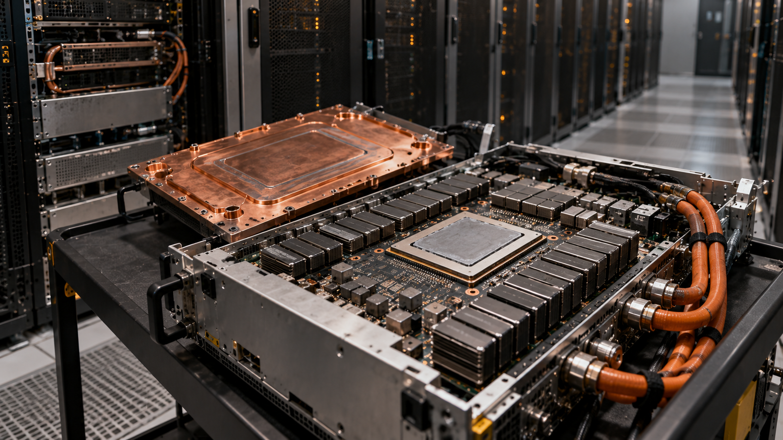
An accelerator bills the same whether it is generating tokens or waiting for a database query to return. The hardware cost is fixed the moment you provision it. The useful work is not.

That asymmetry is the whole subject. Every hour an accelerator spends idle, stalled or doing work that produces no billable output still has to be paid for, and the only place that cost can go is into the price of the tokens the fleet does produce. Accelerator utilisation is therefore not a monitoring metric that sits beside cost. It is a term in the cost equation.

What makes it difficult is that the number most teams watch — the utilisation percentage on the dashboard — answers a narrower question than they think, and the gap between a busy accelerator and a productive one is where inference budgets quietly go.

Key takeaways

• The standard GPU utilisation figure measures the fraction of time at least one kernel was executing. It says nothing about how much of the chip that kernel used, which is why a memory-bound decode step can read 100% while running at a small fraction of peak throughput.
• Prefill and decode stress different parts of the hardware, and mixing them on one pool means one phase interferes with the other. Long prefills stall active decode streams, which is why chunked prefill and disaggregation exist.
• Some idle capacity is deliberate. Queueing delay rises sharply as a system approaches saturation, so latency-sensitive services must hold headroom to protect p95 and p99. A fleet at 60% may be correctly sized and one at 95% may be missing its SLA.
• Agentic workloads break the batching assumption. Between model calls an agent waits on tools, APIs and networks, producing request-level gaps that conventional high-volume batching handles poorly.
• Continuous batching recovers scheduling gaps, disaggregation recovers phase interference, and capacity pooling recovers demand variance. They address different losses and are not substitutes.
• Cost per accelerator-hour is not cost per useful token. The same hour, at different achieved throughput, produces order-of-magnitude differences in effective cost.

---

Quick Navigation

---

The Accelerator Utilisation Number Most Teams Read Incorrectly

Accelerator utilisation, as commonly reported, measures the percentage of time over a sampling period during which one or more kernels were executing on the device. NVIDIA’s own definition is a duty cycle. It is a measure of when, not of how much.

That distinction matters more than it sounds. A kernel occupying a single streaming multiprocessor for the entire sampling window reports the same figure as one saturating every SM on the chip. The metric cannot tell them apart, because it was never designed to.

Five quantities get conflated under the word utilisation, and separating them is the first practical step:

Term	What it means
Theoretical capacity	What the hardware could produce at peak — FLOPS, memory bandwidth, the specification numbers
Allocated capacity	What has been assigned or reserved to a workload, whether or not it is being used
Instantaneous utilisation	The duty-cycle percentage on the dashboard right now
Achieved throughput	Tokens or requests actually produced per second
Economically useful utilisation	The share of accelerator-time that produced output someone is paying for

The last row is the one that appears on the invoice and on no dashboard by default.

Deeper counters help. DCGM exposes SM activity, SM occupancy and Tensor Core pipe activity alongside the basic figure, and research comparing them has shown that the coarse utilisation metric and SM-level activity do not always agree. Tensor Core activity in particular sits closest to the work that produces model output for matrix-heavy inference.

Even those are counters rather than verdicts. A kernel running at a small fraction of peak FLOPS for 100 milliseconds still scores fully on SM activity for that interval.

---

Why an Accelerator Can Be Busy Without Being Efficient

There are several ways to post an impressive utilisation figure while producing very little.

• Memory-bandwidth saturation. A kernel streaming more data than the compute units can consume keeps the SMs occupied while the arithmetic sits idle waiting on HBM. This is the normal state of autoregressive decoding, not an exotic failure. We worked through the memory side of this in our breakdown of what AI memory actually costs, and the short version is that bandwidth, not FLOPS, sets the ceiling for token generation.
• Small batches. A batch of one keeps the device busy and wastes most of its parallelism. The weights must be read from memory for every forward pass regardless of how many sequences ride along, so a batch of one pays the full memory cost for a single token.
• Padding. Batching sequences of unequal length means computing over padding tokens that produce nothing.
• Speculative work that gets discarded. Rejected draft tokens in speculative decoding consumed real cycles.
• Communication and synchronisation. In multi-GPU serving, time spent in collectives or waiting on a peer is time the accelerator is occupied and unproductive.

The common thread: the duty-cycle metric counts occupancy, and occupancy is not output. The question worth asking of any inference fleet is not how busy the accelerators are but how many useful tokens each accelerator-hour produced.

---

Prefill and Decode Pull Accelerator Utilisation in Two Directions

LLM inference runs in two phases with different hardware appetites.

• Prefill processes the input prompt. Every token is available at once, so attention and the feed-forward layers run as large dense matrix multiplications across the whole sequence. This is highly parallel work that can keep arithmetic units genuinely busy.
• Decode generates output tokens one at a time. Each step depends on the previous one, so the parallelism across the sequence disappears. The step reads the model weights and the accumulated KV cache to produce a single token per sequence.

The usual shorthand is that prefill is compute-bound and decode is memory-bound. It is a good first approximation and a poor absolute rule.

Where it breaks down: a very short prompt does not saturate compute during prefill. A large enough decode batch, with many sequences advancing together, reaches arithmetic intensity high enough that compute matters again. Mixture-of-experts routing changes the picture further, and quantisation shifts where the bottleneck falls. The phases have tendencies, and the tendencies are strong enough to design around, but a specific workload on specific hardware can sit anywhere along the spectrum.

What is reliably true is that the two phases interfere when they share a device. A long prefill occupies the accelerator for a substantial block of time, and every decode stream already in flight stalls while it runs. The user sees it as a pause mid-generation — inter-token latency spiking for reasons unrelated to their own request.

The standard mitigation is chunked prefill: split a long prompt into chunks, commonly 512 tokens, and interleave them with decode iterations. Larger chunks mean fewer but longer stalls; smaller chunks mean more but shorter ones. NVIDIA’s tuning documentation for disaggregated serving describes exactly this trade-off, noting that the maximum token setting controls the longest prefill that can be piggybacked onto decode and therefore controls inter-token latency.

This is why a fleet can show healthy utilisation and still fail its latency targets. The accelerators are busy. They are busy doing prefill work that is delaying token generation for everyone else on the device.

---

Traffic Peaks Are the Hidden Accelerator Utilisation Tax

Demand for an inference service is almost never flat. It moves with the working day, with time zones, with weekdays against weekends, with product launches and marketing campaigns, and with whatever a large customer decided to run this morning.

Accelerator capacity does not move with it. You provision a number of devices, and that number is the same at 3am as at 3pm.

The consequence is arithmetic rather than engineering. A fleet sized for peak has unused capacity at every other hour, and the ratio between peak and trough sets a ceiling on average utilisation that no amount of serving optimisation can lift. If peak traffic is three times the trough and you must serve peak, average utilisation over the day cannot approach 100% no matter how good the scheduler is.

Capacity headroom is the deliberate gap between provisioned capacity and expected load. It exists for two reasons: to absorb traffic above forecast, and to keep queueing delay within bounds.

The options for handling variance each carry a different cost:

Approach	What it costs
Size for peak	Idle capacity at every non-peak hour
Size for average	SLA violations during spikes
Autoscale	Cold starts, model loading time, and capacity that may not be available on demand
Pool with flexible workloads	Complexity and isolation concerns

Model loading deserves a note, because it is what makes inference autoscaling harder than web autoscaling. Bringing a new accelerator into service means loading tens or hundreds of gigabytes of weights before it can serve a single token. That delay sits between the spike and the response to it.

---

The Latency SLA That Looks Like Waste

Queueing theory gives the uncomfortable result that makes low utilisation rational.

As a system’s arrival rate approaches its service capacity, queue length and waiting time do not rise linearly. They rise sharply, and near saturation they rise without bound. The practical version: a system running at 70% of capacity has modest queueing delay, and the same system at 95% has delay that dominates the response time entirely.

For a latency-sensitive inference service, that shape sets a hard limit on how high utilisation can go. If your contract or your product requires a p99 time-to-first-token under some threshold, you cannot run the fleet near saturation, because the tail is precisely what breaks first.

This reframes what a dashboard is showing you. Idle capacity on a latency-sensitive service is not necessarily waste. It is the buffer that keeps p95 and p99 within bounds, and removing it converts an accelerator-cost saving into an SLA breach.

A fleet at 95% utilisation is not automatically healthier than one at 60%. The 60% system may be correctly sized for its tail-latency commitment; the 95% system may be quietly missing it. Neither number means anything without the latency distribution beside it.

The corollary is worth stating plainly: utilisation targets should differ by workload class. Batch scoring, overnight document processing and offline evaluation can and should run close to saturation, because nobody is waiting. Interactive serving cannot. Treating both with one utilisation target guarantees you are either wasting money on the batch fleet or breaking the interactive one.

---

Why Agents Create Empty Accelerator Time

A conventional inference request arrives, gets served and leaves. An agent request does something else.

A typical agent turn looks like this:

1. Call the model to decide what to do
2. Wait for a tool — a search, a database query, an API call
3. Receive the result
4. Call the model again with the result in context
5. Wait for another service
6. Call the model once more to produce the answer

Steps 2 and 5 are the problem. During those waits, that request needs no accelerator time at all, but it holds state: its KV cache is either kept resident, occupying memory that could serve another request, or evicted and recomputed later at compute cost.

The waits are not short. A database query takes tens of milliseconds, an external API call hundreds, a web search or a code-execution sandbox longer still. Set against a decode step measured in single-digit milliseconds, a single tool call can be worth hundreds of decode iterations.

Three properties make agent traffic harder to batch than conventional inference:

1. Arrival patterns are bursty and correlated. Many agents hitting step 4 at the same moment creates a spike; the tool waits between steps create troughs. The load is lumpy at exactly the timescale batching operates on.
2. Context grows through the turn. Each step carries the accumulated transcript, so prefill cost rises with every iteration. Late steps in a long agent turn are expensive to re-prefill and expensive to keep cached.
3. Step counts vary wildly. One task finishes in two model calls, another takes twenty. Capacity planning against an average here is planning against a number that describes almost none of the traffic.

None of this means agent workloads necessarily run at poor utilisation. A service with enough concurrent agents can fill the gaps from one agent’s tool wait with another agent’s model call, and prefix caching substantially reduces the cost of re-sending a growing transcript. The difficulty is concentration: a handful of high-value agents produces far worse utilisation than thousands of chat users generating the same token volume, because there is nothing to interleave.

The practical implication is that agent platforms should measure accelerator utilisation against model-call time, not against wall-clock request duration. A request that takes 40 seconds and uses four seconds of accelerator time is not a utilisation failure. Counting it as one leads teams to optimise the wrong layer.

---

Three Ways to Recover Accelerator Utilisation

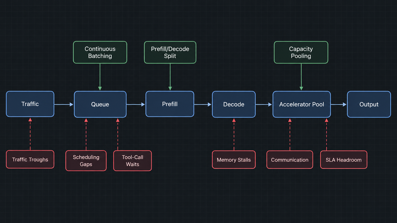
Each mechanism addresses a different loss. Applying one to a problem caused by another wastes engineering time and changes nothing on the invoice.

Continuous batching

Continuous batching works by deciding batch membership at every model iteration rather than once per batch. A finished sequence is evicted immediately and a waiting request takes its slot on the next iteration, so the accelerator does not sit half-empty waiting for the slowest sequence to complete.

The problem it solves is specific to autoregressive generation. Requests in a batch finish at different times because output lengths vary, sometimes by a factor of ten. Under static batching, a batch of 32 where 30 sequences finish at 50 tokens and 2 run to 500 leaves the accelerator computing over 30 empty slots for the remainder — and new arrivals wait for the whole batch to drain, inflating time-to-first-token.

The technique came from the Orca paper at OSDI 2022, which introduced iteration-level scheduling and reported a 36.9x throughput improvement over FasterTransformer at comparable latency. Anyscale’s later benchmarking measured up to 23x over static batching using vLLM, with the additional gains coming from the memory management that iteration-level scheduling makes possible. It now ships by default in vLLM, SGLang and TensorRT-LLM, where it is sometimes called in-flight batching.

The trade-off is latency variance. Higher batch occupancy means more sequences sharing each forward pass, which raises throughput and can raise per-token latency for any individual stream. Long prefills can still stall decode, which is what chunked prefill addresses.

If you are running a serving stack from the last few years, you already have this. The remaining question is whether its settings — maximum concurrent sequences, chunk size — match your traffic.

Prefill-decode disaggregation

Disaggregation separates the two phases onto different accelerator pools. Prefill workers process prompts, transfer the resulting KV cache to decode workers, and the decode pool generates tokens.

The argument for it follows directly from the phase behaviour. Each pool can be sized, tuned and even hardware-matched for one job instead of compromising between two, and long prefills stop interrupting decode streams because they are happening on different devices.

The cost is the transfer. Every request’s KV cache must move from the prefill pool to the decode pool, and that state is large. NVIDIA’s Dynamo uses NIXL to move KV tensors directly between the VRAM of the prefill and decode engines over NVLink or InfiniBand, with the transfer non-blocking so the forward pass can continue serving other requests during it. The engineering effort visible in that design — topology-aware placement to keep transfers inside a network domain, proposals to transfer only the KV blocks a decode worker does not already hold — is a reasonable indicator of how much the transfer cost matters.

Disaggregation is not universally better. It adds a routing layer, a transport dependency and a second pool to operate and capacity-plan. It pays off most clearly at scale, with high input-to-output token ratios such as RAG and summarisation, and where prefill interference is measurably hurting inter-token latency. For a single-node deployment serving moderate traffic, the complexity usually is not worth it.

Capacity pooling

The third mechanism attacks demand variance rather than serving mechanics: put more workloads on the same capacity so the troughs of one fill the peaks of another.

Approaches that work in practice:

• Multi-tenant serving, where many customers or internal teams share a fleet, smoothing individual variance
• Model sharing, serving several fine-tunes as adapters over one resident base model rather than loading each separately
• Flexible workload scheduling, running batch jobs, evaluation and offline scoring in the gaps left by interactive traffic
• Geographic pooling, where time-zone offsets mean one region’s trough coincides with another’s peak
• Routing, directing requests to the pool with capacity and the right cached prefix

The trade-offs are real and belong in the decision:

Benefit	Cost
Smoothed demand	Noisy neighbours affecting tail latency
Higher average utilisation	Isolation and data-residency constraints
Better amortisation of loaded models	Cold starts when switching models
Absorbed spikes	Routing complexity and a new failure domain

For regulated workloads, isolation requirements may rule out pooling entirely, and that constraint is not negotiable against a utilisation target. Where pooling is available, it is often the largest single improvement, because demand variance is usually the biggest source of idle capacity — and unlike the other two mechanisms, it needs no change to the serving stack.

---

Turning Accelerator Utilisation Into Cost Per Token

The chain from hardware to invoice runs like this:

Accelerator cost → available capacity → achieved throughput → utilisation → cost per token → cost per request

The first term is fixed. Whether you rent by the hour or amortise a purchase, that number does not change with how busy the device is. Everything downstream is variable, which means all the variance in cost per token comes from the right-hand side of the chain.

The arithmetic that matters:

Cost per million tokens = (accelerator hourly cost ÷ tokens produced per hour) × 1,000,000

Here is what that does in practice. Every figure below is an illustrative assumption, not a vendor quote or a measured benchmark. Assume an accelerator costing $3.00 per hour and a model that, at full batch occupancy on that device, could produce 3,000 output tokens per second.

Scenario	Achieved tokens/sec	Tokens/hour	Cost per 1M output tokens
Batch size 1, no batching	90	324,000	$9.26
Static batching, partly drained batches	750	2,700,000	$1.11
Continuous batching, steady traffic	2,400	8,640,000	$0.35
Continuous batching, 40% duty cycle from demand troughs	960	3,456,000	$0.87

Same hardware. Same hourly price. A 26x spread in effective cost, driven entirely by how much useful work each hour contained.

Two things in that table are worth dwelling on. The jump from row one to row three is what serving-stack improvements buy. The drop from row three to row four is what demand variance takes back — and notice that the fourth row has an excellent serving stack and still costs 2.5x the third, because the accelerators are idle 60% of the time.

That is the argument for treating utilisation as an economic variable rather than an ops metric. A team that has already deployed continuous batching can still be paying multiples of its theoretical cost floor, and no serving-layer optimisation will fix it. The remedy is pooling, scheduling or right-sizing.

The cost-per-token framework itself — input against output pricing, cache reads, the difference between token cost and cost per completed task — we set out in our breakdown of what inference actually costs per token. Utilisation is the multiplier sitting underneath all of it, and where it fits in the broader infrastructure picture is covered in our map of the AI compute stack.

One caution about the table above: it models output tokens only. Real workloads pay prefill cost too, and for RAG or long-context traffic prefill can dominate. A complete model needs both, which is why the measurement section below asks for input and output token counts separately.

---

What Your Accelerator Utilisation Dashboard Should Show

One number cannot carry this. A usable view needs six groups, and they answer different questions.

Group	Metrics	The question it answers
Capacity	Devices provisioned, devices allocated, devices serving	How much hardware exists and how much is assigned
Activity	GPU utilisation, SM activity, SM occupancy, Tensor Core activity, memory used, achieved memory bandwidth	How busy the silicon is, and at what depth
Throughput	Output tokens/sec, input tokens/sec, requests/sec, batch size	How much work is coming out
Latency	TTFT, inter-token latency, p50, p95, p99, queue time	Whether the service is meeting its commitments
Cost	Cost per request, cost per million tokens, useful work per accelerator-hour	What it is actually costing
Idle	Time attributed to each idle category below	Where the lost capacity went

The idle breakdown is the part most teams do not have, and it is the one that tells you what to fix. Categorise it:

• No demand — nothing to serve. Fix with pooling, scheduling or right-sizing.
• Queueing and scheduling gaps — work waiting while the device is not full. Fix at the scheduler.
• Tool-call waits — agent requests holding state while external services respond. Fix with concurrency or cache policy.
• Memory stalls — compute waiting on HBM. Fix with batching, quantisation or better kernels.
• Communication — collectives and transfers in distributed serving. Fix with topology and parallelism strategy.
• Model loading — cold starts and weight loading. Fix with warm pools or adapter sharing.
• Failures and retries — work done twice or thrown away.
• SLA headroom — deliberate. Do not fix; label it and defend it.
• Orchestration overhead — time in your own routing and serving layers.

The last category on that list is the reason the exercise is worth doing. Without it, every idle minute looks identical on a graph, and the team optimises whichever cause it happened to guess.

---

A 50-Request Test You Can Run This Week

Take 50 to 100 requests that look like your real production traffic — not curated examples, not the happy path — and replay them against your serving stack while recording everything.

Per request, capture: input tokens, output tokens, TTFT, total latency, queue time, batch size at admission, tool-call waiting time where relevant, retries, failures, and the cost computed from your own hourly rate.

Across the run, capture: p50, p95 and p99 latency, aggregate tokens per second, accelerator utilisation, SM activity, and achieved memory bandwidth.

Then read the results against this table, which is how you turn the numbers into a decision:

What you observe	Likely bottleneck	Where to look
Low utilisation, low queue time	Insufficient demand	Pooling, scheduling, fleet size
Low utilisation, high queue time	Scheduling or admission	Batching configuration, concurrency limits
High utilisation, low throughput	Memory bandwidth or small batches	Batch size, quantisation, kernel efficiency
High TTFT, acceptable inter-token latency	Prefill contention or queueing	Chunked prefill, disaggregation
Inter-token latency spikes mid-generation	Long prefills interrupting decode	Chunked prefill, prefill routing
Utilisation swings hour to hour	Demand variance	Pooling, autoscaling, batch backfill
Long wall-clock time, low accelerator time	Agent orchestration and tool latency	Not an accelerator problem — look at the tools
High retry rate	Errors, timeouts, capacity limits	Serving errors, admission control

Fifty requests will not give you statistical confidence. They will give you the shape of the distribution and a defensible answer to the only question that matters at this stage: which layer is actually costing you money. Run it again after every change, because the bottleneck moves.

---

What Accelerator Utilisation Can and Cannot Tell You

It can tell you whether hardware is sitting completely idle, which is worth knowing and easy to act on.

It can, read over time, show you the shape of your demand and therefore how much of your bill is structural rather than technical.

It cannot tell you whether the work being done is useful, whether the chip is being used efficiently while busy, or whether your latency commitments are being met. For those you need throughput, the deeper activity counters and the latency distribution.

The useful mental shift is to stop treating utilisation as a health metric and start treating it as a cost variable — one that can be moved deliberately, in known directions, by known techniques, with known trade-offs:

• Scheduling gaps → continuous batching
• Phase interference → chunked prefill, then disaggregation if the scale justifies it
• Demand variance → pooling, flexible workload scheduling, right-sizing
• Tail-latency headroom → leave it alone and label it

A fleet running at 55% because it protects a p99 commitment and backfills nothing is telling you something specific: there is money on the table, and it is in the backfill, not the serving stack. A fleet at 90% with poor throughput is telling you something different. The number alone says neither.

---

Frequently Asked Questions

---

Keep reading

Here are the latest posts from the blog.