Kimi K3.1 Pro Hardware Requirements: GPUs, Memory, Cost

Kimi K3.1 Pro hardware requirements

Last updated: 5 November 2026. Kimi K3.1 Pro’s official weights are now on Hugging Face, so we’ve confirmed the parameter count, expert layout, MXFP4 format and checkpoint size, replaced the K3 licence terms with the published K3.1 Pro licence, corrected the attention layout and added a section on downloading the weights safely.

Before anyone argues about which GPU to rent, a smaller question settles most of the argument: how many bytes have to sit in accelerator memory before the first token comes out? For Kimi K3.1 Pro hardware requirements, that number already exists, even though the model’s own weights don’t.

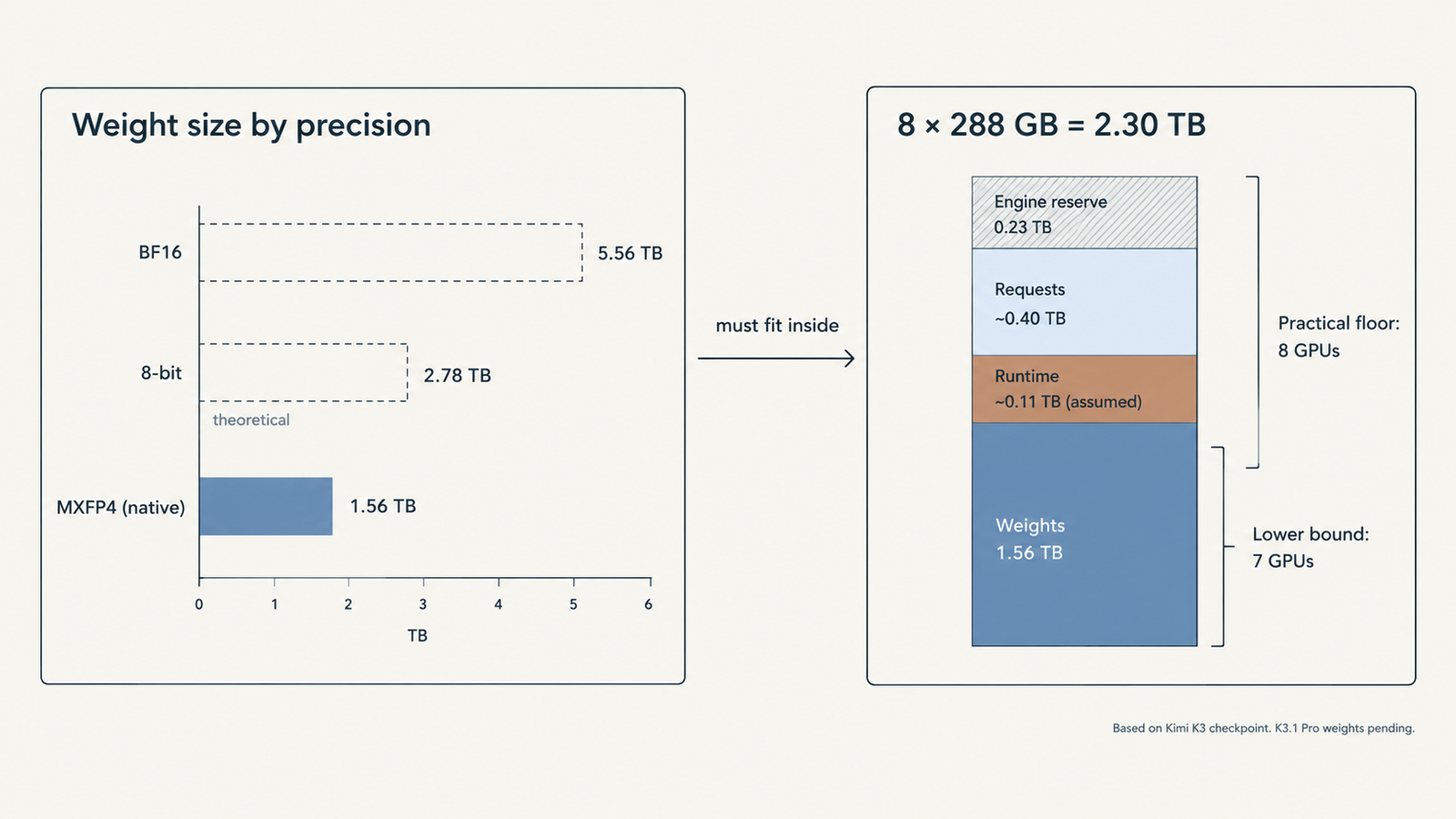
Moonshot AI launched Kimi K3.1 Pro on its API on 23 October and describes it as a post-trained version of Kimi K3. K3’s weights have been public since July, and they occupy 1.561 TB. Unless Moonshot changes the format when it publishes K3.1 Pro, that’s the floor: about 1.56 TB of weights before a single cached token, activation buffer or draft model.

A model name doesn’t give you a GPU count. Weight format, memory per accelerator, the engine’s reservation, context length and concurrency do. This guide works through each with the arithmetic shown, so you can swap in your own numbers.

Quick Answer
  • Weights released: Kimi K3.1 Pro’s official weights went live on Hugging Face at the start of November 2026, under the moonshotai organisation.
  • Model size: 2.8T total parameters with 104B active, shipped as a 1.56 TB MXFP4 checkpoint split across 96 files.
  • Memory needed: about 1.6 TB of GPU memory for the weights alone, before KV cache.
  • Minimum GPUs: eight 288 GB GPUs (B300, GB300 or MI355X) as a floor, 16 B200 or H200 cards, or 24 to 32 H100s. These are our estimates, since Moonshot publishes no minimum hardware.
  • Long context: the 1M-token window adds up to about 18 GB per request on our revised estimate.
  • Licence: the Kimi K3.1-Pro License is MIT-style, with extra conditions above $20M in revenue or 100M monthly users.
  • Download safely: use only the official moonshotai repository and verify the files before you load them.
Key Takeaways
  • The official weights are out: 2.8T total parameters, 104B active, 1.56 TB across 96 safetensors shards on Hugging Face.
  • Fake and repackaged Kimi K3.1 Pro uploads are likely to follow, so download only from the moonshotai organisation and verify model weights before you download.
  • “2.8 TB at 8-bit” is arithmetic for a file that doesn’t exist. The native release is already 4-bit, trained that way.
  • Eight 288 GB GPUs in one node are the floor. B200, H200 and H100 fleets need two or more nodes just to hold the weights.
  • Every request costs a fixed 0.2 to 0.4 GB of KDA state plus about 14 KB per token of FP8 MLA cache, so short requests aren’t as cheap as their length suggests and million-token contexts are cheaper than on dense models.
  • A single on-demand AWS node costs about $102,540 a month before redundancy, staff or storage.
  • Matching the $2/$10 API on a 20k-in, 2k-out workload takes roughly 13,000 input and 1,300 output tokens per second, sustained around the clock. Measure whether your hardware can do that before you sign anything.
  • The K3 licence isn’t MIT: model-as-a-service businesses above $20 million in total company revenue need a separate agreement.

Quick Navigation


What is confirmed about Kimi K3.1 Pro

With the weights released on Hugging Face, every core specification on this page now comes from Moonshot’s own model card and config.json rather than from Kimi K3.

SpecificationKimi K3.1 ProSource
Total parameters2.8TModel card
Active parameters per token104BModel card
Layers93 (1 dense)Model card
Attention layout69 KDA (linear attention) + 24 Gated DSA (sparse attention)Model card, config.json
Experts896, with 16 routed + 2 shared per tokenconfig.json
Hidden size / attention heads7168 / 96Model card
Weight formatMXFP4 weights, MXFP8 activations, quantization-aware trainingModel card
Context window1,048,576 tokensconfig.json
Vision encoderMoonViT-V2, 401M parametersModel card
Checkpoint size1.56 TB, 96 safetensors shardsHugging Face file tree
Recommended enginesvLLM, SGLang, TokenSpeedModel card
APILive as kimi-k3.1-proKimi blog

One change from Kimi K3 matters for memory planning. K3.1 Pro swaps K3’s 24 full-attention Gated MLA layers for Gated DSA, a sparse attention design, which changes the KV cache figures below. Moonshot doesn’t state minimum hardware anywhere in the release, so the GPU counts on this page remain our estimates from the published sizes.

Calculating Kimi K3.1 Pro weight memory
Kimi K3.1 Pro hardware requirements

The formula is plain: weight bytes = parameters x bits per parameter ÷ 8. Using K3’s 2,779,931,837,184 parameters:

PrecisionBits per parameterDecimal TBBinary TiBWhat it represents
BF16165.5605.057Theoretical; no such release
8-bit (FP8/INT8)82.7802.528Theoretical
4-bit, no scales41.3901.264Theoretical minimum
MXFP4 everywhere4.251.4771.343Adds one 8-bit scale per 32 weights
Actual K3 checkpoint4.49 (effective)1.5611.420Published repository, 96 shards

The released checkpoint confirms the MXFP4 estimate. Moonshot’s config lists the format as mxfp4-pack-quantized with one scale per group of 32 weights, and the Hugging Face repository totals 1.56 TB across 96 shards. Plan for about 1.6 TB of memory for weights, plus room for the vision encoder, KV cache and runtime overhead.

All rows are weights only, with no runtime overhead. The brief’s “2.8 TB at 8-bit, 1.4 TB at 4-bit” is correct arithmetic for the wrong question. Moonshot trained K3 to run in MXFP4 from supervised fine-tuning onward, so there is no 8-bit release to plan around.

The gap between 1.39 TB and 1.561 TB has two sources. MXFP4 stores a shared 8-bit scale for every block of 32 weights, adding about 0.09 TB. And the config leaves attention, shared experts, the dense first-layer MLP, the output head and the vision encoder unquantized. The “5.6 TB” figures circulating for K3 come from assuming BF16.

Watch your units. TB is 10^12 bytes and TiB is 2^40, about 10% larger. NVIDIA lists a DGX B300’s total GPU memory as “2.1 TB”, yet eight 288 GB GPUs hold 2,304 GB, which is 2.10 TiB. Compare a TiB capacity with a TB weight file and you’ve lost a tenth of your headroom on paper.

How many GPUs Kimi K3.1 Pro needs

The lower bound is: GPUs = ceiling(weight bytes ÷ (memory per GPU x usable fraction)). vLLM’s Kimi K3 recipes run at 0.88 to 0.92 of GPU memory; this guide uses 0.90.

AcceleratorMemory per GPULower boundPractical layoutFits one 8-GPU node?
NVIDIA B300 / GB300288 GB78Yes, ~513 GB left after weights
AMD MI355X288 GB78Yes, same arithmetic
NVIDIA B200180 GB1016 (two nodes)No: 1,440 GB total
NVIDIA H200141 GB1316 (two nodes)No: 1,128 GB total
NVIDIA H10080 GB2224 to 32 (three to four nodes)No

Memory per GPU from AMD’s MI355X page (which also lists B200 at 180 GB) and NVIDIA. Seven 288 GB GPUs clear the bound, but tensor parallelism splits the 96 attention heads across GPUs, and 96 doesn’t divide by seven. Eight is the real floor, and it’s what the vLLM recipe states: at least 8x GB300, or 8x MI355X/MI350X on ROCm, with “multi-node for real production traffic”.

Eight GPUs are not one 2.3 TB pool. Each holds its own shard, and every layer exchanges activations between them. Inside a DGX B300 that traffic rides NVLink at 14.4 TB/s aggregate. Between nodes it crosses InfiniBand or Ethernet at up to 800 Gb/s per port, roughly 100 GB/s, which is why two-node recipes split the model into pipeline stages (TP8 x PP2) and why NVIDIA’s Dynamo recipes target GB200 and GB300 racks with NVLink spanning trays: 16 GB200s aggregated, or 32 split between prefill and decode.

Hopper is the awkward case. H100 and H200 lack native FP4 tensor cores, so MXFP4 experts run through dequantising kernels. The recipe page builds commands for H200, but its stated minimum is Blackwell or MI355X, and we found no published throughput for K3 on Hopper.

Can a single GPU or workstation run it?

No single GPU comes close. The workstation route is llama.cpp with the experts in system RAM. One published test loaded a ~554 GB 1-bit GGUF of K3 on a 160 GB VRAM machine with the MoE weights on CPU. Nobody has published quality figures for that quant. The 4-bit GGUF is 1,508.7 GB, barely smaller than the native file, because the native file is already 4-bit. It’s a way to poke at the model, not to serve users, and Now that the weights are public, community quants of Kimi K3.1 Pro can appear, but none are official, and their quality and memory use are unverified until someone tests them. The K3 result above (a 554 GB 1-bit GGUF reportedly running on 160 GB of VRAM) is the best guide for now. Before you run any community build, put it through the checks in our model weights verification guide..

The KV cache changes the Kimi K3.1 Pro calculation

This is the one part of the page where the release changed our numbers. Our first estimate assumed K3’s Gated MLA layers. Kimi K3.1 Pro uses Gated DSA in those 24 layers instead, and its config gives the inputs for a revised estimate.

  • DSA layers: the config keeps a 512-value compressed KV latent plus a 64-value positional key (576 values), and adds a lightning indexer with a 128-dimension key. Assuming each of the 24 layers caches both, as DeepSeek’s DSA does, that’s 24 × (576 + 128) = 16,896 values per token, or about 16.9 KB at FP8.
  • KDA layers: these keep a fixed-size state rather than a growing cache. At 69 layers × 96 heads × 128 × 128 values in BF16, that’s about 0.22 GB per request, whatever the context length.
Context lengthDSA cache (FP8)KDA stateTotal per request (estimate)
8K tokens0.14 GB0.22 GB0.36 GB
32K tokens0.55 GB0.22 GB0.77 GB
128K tokens2.21 GB0.22 GB2.43 GB
256K tokens4.43 GB0.22 GB4.65 GB
1M tokens17.72 GB0.22 GB17.93 GB

Treat these as planning estimates, not measured figures. Moonshot hasn’t published KV cache sizes, and vLLM or SGLang may store the cache differently. The indexer only picks the top 2,048 earlier tokens for each query (index_topk in the config), which saves compute, but the full cache still has to sit in memory. Check your engine’s own memory report once the model loads.

Two things fall out. Below about 16,000 tokens the fixed state outweighs the growing cache, so short chat traffic carries a per-request floor most sizing guides ignore. At the other end, long contexts are cheap: a 70B dense model with grouped-query attention needs about 160 KB per token, as our breakdown of AI memory costs works out, or roughly 172 GB for a million tokens against K3’s 14.7 GB.

On one 8x B300 node, 0.90 of 2,304 GB leaves about 2,074 GB, and weights take 1,561 GB. Set aside an assumed 110 GB for activations, CUDA graphs, communication buffers and the speculative draft model the recipes load, and roughly 400 GB remains for requests. That’s an upper bound of about 600 concurrent requests at 32K, 197 at 128K, or 27 at the full million.

Those counts assume the cache is spread across GPUs without duplication. vLLM’s decode context parallelism does that for MLA; without it, tensor-parallel ranks can each hold a copy and the numbers fall sharply. The recipes also spill to host RAM: one AMD prefill configuration budgets 1,799 GB of host DRAM for cache offload. Memory scales linearly with concurrency and context. Throughput at those concurrencies is a separate question that only measurement answers.

Where to download Kimi K3.1 Pro weights safely

The only official source is the moonshotai/Kimi-K3.1-Pro repository on Hugging Face. A 1.56 TB download is a big target for copycats, and a fake or tampered upload costs you days of transfer time and GPU hours before you notice anything is wrong.

There’s a second reason to be careful with this release. The repository ships its own Python files, and Moonshot’s usage example loads them with trust_remote_code=True. A mirror that changes those files can run code on your servers the moment you load the model. Our guide to spotting fake model weights walks through seven checks before you download. For Kimi K3.1 Pro, the short version is:

  1. Check the organisation. The repo should sit under moonshotai, the same Hugging Face account that hosts Moonshot’s earlier Kimi K3 release.
  2. Check the file list. Expect 96 safetensors shards totalling about 1.56 TB, plus config.json, the LICENSE and the custom code files. Pickle or .bin weight files are a warning sign.
  3. Read the custom code before you trust it. If you pull from anywhere other than the official repo, compare the .py files against Moonshot’s versions line by line.
  4. Compare hashes. Hugging Face shows a SHA-256 for each large file. Match your local copies against the official repo, not against the mirror you downloaded from.
  5. Treat quants as third-party software. Moonshot hasn’t released any official quantised variants. Any GGUF or lower-bit build is a community conversion, so check who made it and what it was built from.

Quantisation trade-offs

Weight quantisation and cache quantisation are separate levers, and the first one is mostly pulled already.

LeverMemory effectWhat you risk
Keep native MXFP4 weightsBaseline 1.561 TBNothing; this is how the model was trained
Up-cast to FP8 or BF161.8x to 3.6x moreHardware cost, with no documented quality gain
Community 1-bit or 2-bit quantsAbout 0.55 TB for the smallest published 1-bit GGUFUnmeasured quality loss; K3-only until K3.1 Pro weights ship
FP8 KV cacheHalves the MLA cache versus BF16Small accuracy risk; recipes use it by default
FP32 vs BF16 KDA stateDoubles or halves the fixed per-request stateSome low-latency backends require FP32

Because K3 went through quantization-aware training, its 4-bit weights aren’t a lossy copy of some better original that’s available to you. Going below 4 bits is a real compression, and nobody has published K3 or K3.1 Pro quality numbers for those quants. Run your own evaluation against the hosted API before trusting one.

Hardware matters here too. Blackwell and AMD’s CDNA 4 parts execute MXFP4 natively; AMD lists 10.1 PFLOPs of MXFP4 matrix throughput for the MI355X. Hopper doesn’t, which is a second reason the recipes start at Blackwell. The cache side has its own knobs: the latency-tuned GB300 profile switches the KDA state to FP32, doubling that per-request floor to about 0.43 GB.

The real cost of self-hosting Kimi K3.1 Pro
Kimi K3.1 Pro hardware requirements

Two dated price points for one 8x B300 node, on demand, 30 days at 24 hours:

ItemAWS p6-b300.48xlargeMedian specialist cloud
Hourly, 8x B300$142.42$65.44 ($8.18 per GPU)
30 days continuous (720 h)$102,540$47,117
Effective rate at 50% useful utilisation$284.83/h$130.88/h
Effective rate at 25% useful utilisation$569.66/h$261.76/h

AWS rate: us-east-1, Linux, on demand, per Vantage’s EC2 tracker, read 26 October 2026; the instance includes 4,096 GiB of host RAM and 8 x 3.84 TB local NVMe. Specialist rate: median across 10 providers per getdeploying, 8 September 2026; those offers may not match AWS on networking, storage or availability.

The effective-rate rows are the ones that matter. A node you pay for around the clock but keep busy half the time costs twice as much per useful hour, and real traffic has nights and weekends.

The GPU line also isn’t the bill. One node has no redundancy, so a production service needs a second, doubling the fixed cost before it serves an extra token. Add engineering time, monitoring, storage for 1.56 TB of weights plus staging on every node, egress, and the work of swapping in K3.1 Pro weights when they arrive. Published estimates of that total put it at 1.3 to 5 times the raw GPU rate, a range we unpack in the hidden fees in self-hosted LLM cost.

Kimi K3.1 Pro API vs self-hosting: the break-even

Moonshot’s API price for standard kimi-k3.1-pro is $2 per million input tokens, $10 per million output and $0.20 per million cached input, confirmed by Artificial Analysis. The Highspeed variant costs $4/$20. Cache writes are billed separately at a rate that wasn’t displayed when we checked.

The formula: API cost = (input tokens ÷ 1,000,000 x input rate) + (output tokens ÷ 1,000,000 x output rate).

Illustrative workload, an assumption: an agentic coding call with 20,000 input tokens and 2,000 output tokens, reasoning included. Uncached, that’s $0.04 + $0.02 = $0.06 per call. With 90% of input served from cache, it’s $0.0076 + $0.02 = $0.0276, before cache-write fees.

Break-even calls per month = monthly self-hosting cost ÷ API cost per call. Spread over 2,592,000 seconds in 30 days:

Scenario (GPU cost only)Calls/month to match APISustained calls/sInput tokens/sOutput tokens/s
AWS, no cache1.71M0.6613,1871,319
AWS, 90% cache hits3.72M1.4328,6672,867
Specialist cloud, no cache785K0.306,059606
Specialist cloud, 90% cache hits1.71M0.6613,1721,317

Caching makes the API cheaper, so it pushes break-even further away. And these are averages held for 720 hours straight. Peaks need headroom above them, so a fleet that just breaks even on average is running below capacity most of the day.

Can one node sustain those rates at an acceptable latency? There’s no independent published throughput for K3.1 Pro on 8x B300, so that’s the number to measure, not assume. Remember too that the right comparison is the cheapest API that meets your quality bar. Third-party hosts listed K3 below Moonshot’s own price on OpenRouter, and the same is likely once K3.1 Pro weights circulate. Our Kimi K3.1 Pro vs Sonnet 5.5 comparison covers per-task token use, which moves the API side of this equation more than the rate card does.

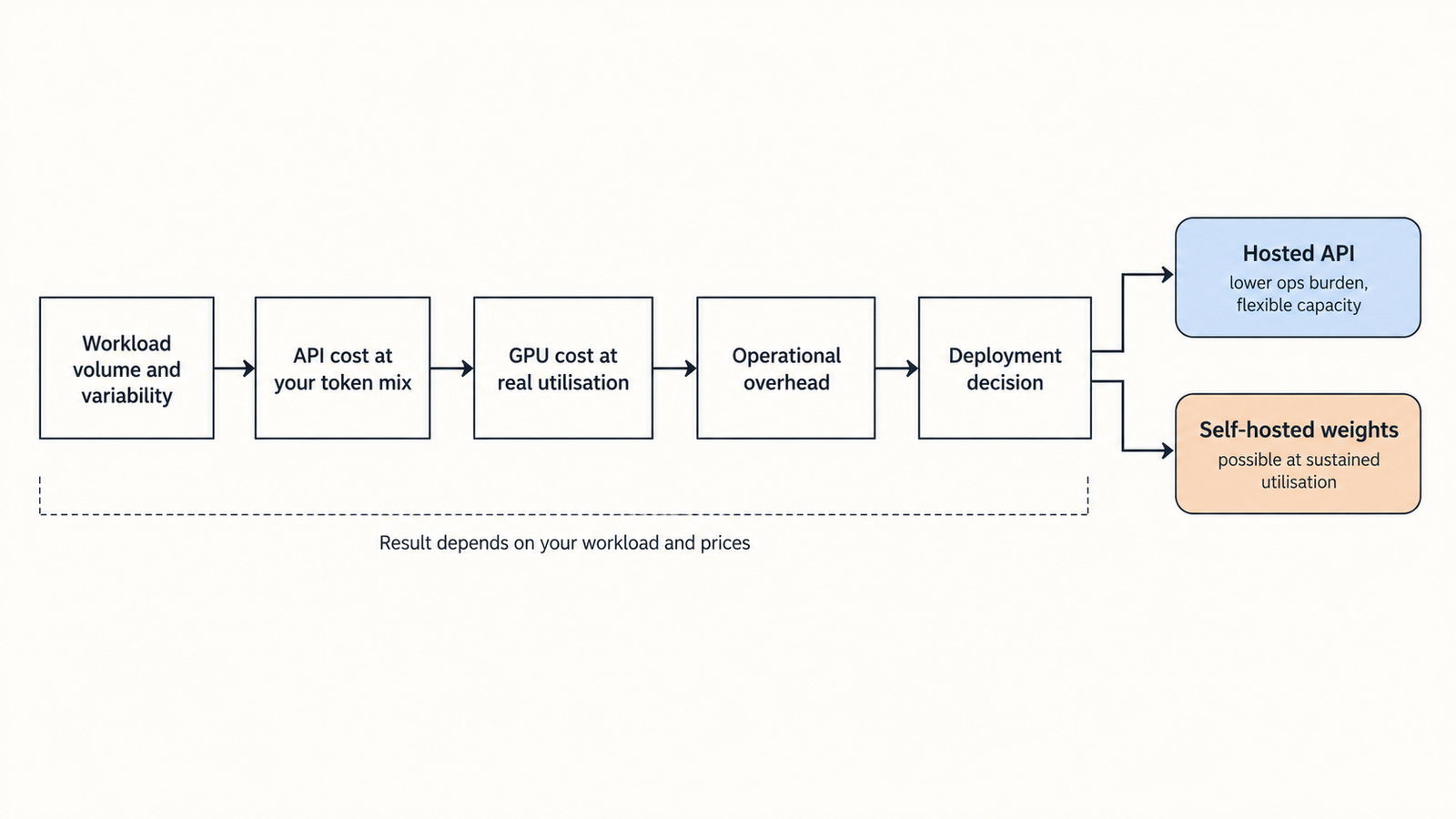
Self-hosting earns its place when data can’t leave your infrastructure, when load is high and steady enough to keep a node busy, when you need to fine-tune, or when you already own Blackwell capacity sitting idle.

Licence and operational constraints

Moonshot published the Kimi K3.1-Pro License with the weights. It starts as an MIT-style licence, then adds three conditions that matter for self-hosting.

  • Model-as-a-Service: if you sell access to the model and earn more than $20M in aggregate revenue over any consecutive 12 months, you need a separate agreement with Moonshot.
  • Attribution: a product with more than 100 million monthly active users, or more than $20M in monthly revenue, must prominently display “Kimi K3.1-Pro”.
  • Exemptions: internal use is exempt, as is use through Moonshot’s official products or certified inference partners.

For most teams running the model in-house, the licence won’t change the hardware decision. If you plan to resell inference at scale, email license@moonshot.ai before you buy GPUs. This is a summary, not legal advice, so have your counsel read the full text.

A practical Kimi K3.1 Pro deployment decision

  • Use the hosted API when traffic is small, spiky or unproven, or nobody on the team runs GPU clusters. Moonshot offers zero data retention to API customers, which settles some privacy objections without any hardware.
  • Rent one 8x B300 or MI355X node for evaluations, fine-tuning experiments or steady internal batch work you can keep busy. Accept that it has no redundancy.
  • Plan multi-node or rack-scale for production with latency targets, long contexts at high concurrency, or uptime commitments. Moonshot’s 64-plus accelerator guidance describes this tier.
  • Benchmark before you sign. Replay 50 to 200 real requests, measure tokens per second at your p95 latency target, and compare any quantised variant’s outputs with the hosted API.

What would change this estimate? The K3.1 Pro file size and precision; the KDA state dtype your engine uses; your measured throughput per node; GPU rental prices, which roughly doubled for B300 through 2026 according to price trackers; and the K3.1 Pro licence terms.

Conclusion

Kimi K3.1 Pro’s weights are now public, and they match the estimates this page made before launch: a 1.56 TB MXFP4 checkpoint that needs about 1.6 TB of GPU memory before KV cache. Eight 288 GB GPUs remain the practical floor, and the 1M-token context adds up to about 18 GB per request on our revised estimate. For most teams the API is still the cheaper route unless usage is heavy and steady. If you do self-host, start from the official moonshotai repository and verify the files before anything touches your cluster.

So don’t rent for Kimi K3.1 Pro hardware requirements yet. Use the API, log your real token mix and concurrency, and when the weights land, check the file size against 1.56 TB, then spend a week on one rented node measuring tokens per second at your latency target. If that number can’t clear the break-even rates in the table above with room for peaks and a second replica, the API was the cheaper machine all along.

Frequently asked questions

How much VRAM does Kimi K3.1 Pro need?

About 1.6 TB for the weights alone, based on the official 1.56 TB MXFP4 checkpoint, plus KV cache and overhead. That’s eight 288 GB GPUs at minimum, 16 B200 or H200 cards, or 24 to 32 H100s. Moonshot doesn’t publish minimum hardware, so these counts are our estimates.

Can Kimi K3.1 Pro run on one GPU?

No. The largest current accelerators, NVIDIA B300 and AMD MI355X, hold 288 GB each, under a fifth of the 1.56 TB weight file. Even heavily compressed community quants of K3 run to roughly 550 GB, which still needs several GPUs or large amounts of system RAM.

How many GPUs are needed for a model of this size?

Eight 288 GB GPUs are the practical minimum and match the vLLM recipe’s stated floor. With 180 GB B200s or 141 GB H200s you need 16 across two nodes. Moonshot recommends 64 or more accelerators for efficient production serving.

Does 4-bit quantisation reduce memory requirements?

For this model it’s already applied. Kimi K3 ships in MXFP4, a 4-bit format with shared scales, trained that way from fine-tuning onward. Converting to 8-bit would roughly double memory. Going below 4 bits shrinks the file further, but no published quality data exists for those quants.

How much does self-hosting cost per month?

One 8x B300 node costs about $102,540 for 30 days on AWS on demand, or about $47,117 at the median specialist-cloud rate (prices checked September to October 2026). Redundancy, staff, storage and idle time add substantially to that GPU line.

Is an API cheaper than running the model locally?

For most workloads, yes. At $2/$10 per million tokens, a self-hosted AWS node only matches the API if it sustains about 1.7 million 20k-token calls a month. Self-hosting can win on data control, steady high load or fine-tuning needs.

Can I run Kimi K3.1 Pro on a workstation?

Not at the official precision. The checkpoint is far larger than any workstation’s memory. Community quants may make heavily compressed versions possible, as a 1-bit GGUF did for Kimi K3, but none are official and quality is untested.

What licence applies to commercial deployment?

The Kimi K3.1-Pro License, an MIT-style licence with extra conditions. Model-as-a-Service businesses earning over $20M in 12 months need a separate agreement, and products above 100M monthly users or $20M monthly revenue must display “Kimi K3.1-Pro”. Internal use is exempt.

Where can I download Kimi K3.1 Pro safely?

Only from the official moonshotai/Kimi-K3.1-Pro repository on Hugging Face. Check the organisation, file list and hashes before downloading, and see our guide to verifying model weights for the full checklist.


Keep reading

AGI vs superintelligence

AGI vs Superintelligence: A New Name Isn’t a New Intelligence
Facts checked against official documents and reporting on 18 November 2026. On 29 September, the White House told federal agencies to stop writing “artificial intelligence” …
AI Coding Agent

AI Coding Agents Are Getting Expensive. Who’s Paying for the Tokens?
Pricing checked on official vendor pages on 17 November 2026. All USD. Cost scenarios are illustrative and labelled as such. On 28 October, TechCrunch published …
Model Weights

Verify Model Weights: 7 Checks Before You Download
Checked against the burner22/numbat repository and its discussions, Hugging Face and PyTorch documentation, and Moonshot AI’s announcement on 2 November 2026. On 1 November, a …
Agentic AI Statistics

30 Agentic AI Statistics for 2026: Adoption, Spending and Risk

Last updated: 15 November 2026. This page is updated monthly; each figure keeps its original publication date. Agent traffic at one healthcare booking platform rose …

Kimi K3.1 Pro vs Sonnet 5.5: Same Price, Different Bill

Kimi K3.1 Pro

On paper, Moonshot AI priced Kimi K3.1 Pro to the cent against Claude Sonnet 5.5: $2 per million input tokens and $10 per million output tokens. Run both through the same independent test suite, though, and the bills part ways. Artificial Analysis spent an average of $2.11 per task running Kimi K3.1 Pro through its Intelligence Index. Sonnet 5.5 at maximum effort cost $5.46 per task on the same evaluations.

The token price is identical. The cost of the work is not, and that gap matters more than any score Moonshot published when it released the model on 23 October 2026.

The second thing to know is that Kimi K3.1 Pro is not yet an open-weight model. Moonshot says the full weights will be released by 4 November. Until they appear, it is a hosted API like Sonnet 5.5, and the questions that come with downloadable weights are still ahead.

This comparison was researched on 26 October 2026. It weighs Kimi K3.1 Pro against Claude Sonnet 5.5 and Claude Opus 5.5 on independently measured capability, list price, measured cost per task, and what changes when weights ship. Provider-reported figures are labelled throughout.

Key Takeaways
  • Kimi K3.1 Pro and Sonnet 5.5 share a $2/$10 list price, but Sonnet 5.5’s cache reads cost $0.10 per million tokens against Kimi’s $0.20.
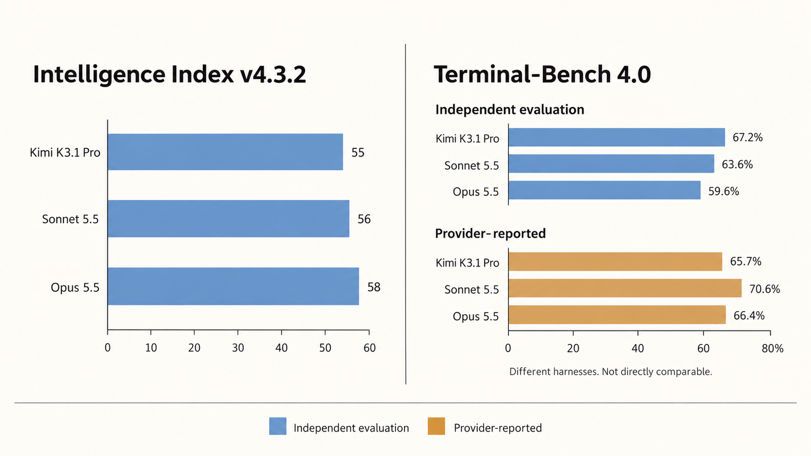
  • On Artificial Analysis’s Intelligence Index v4.3.2, Kimi K3.1 Pro scores 55, Sonnet 5.5 56 and Opus 5.5 58. A one-point gap does not show either model is better.
  • Terminal-Bench 4.0 rankings flip with the harness: vendor numbers put Sonnet 5.5 first, while Artificial Analysis’s run puts Kimi K3.1 Pro first at 67.2%.
  • Kimi K3.1 Pro used about a quarter of Sonnet 5.5’s output tokens per index task at max effort, which is why it cost $2.11 per task against $5.46.
  • Weights are promised by 4 November 2026. Serving 2.8 trillion parameters is a multi-GPU data-centre job, not a workstation install.

Quick Navigation


The price comparison needs a footnote

The list prices are where the “same price” claim holds.

Per 1M tokensInputOutputCache hitCache write
Kimi K3.1 Pro$2.00$10.00$0.20Billed by TTL; rate not displayed at research date
Claude Sonnet 5.5$2.00$10.00$0.10$2.50 (5 min), $4.00 (1 h)
Claude Opus 5.5$4.00$20.00$0.20$5.00 (5 min), $8.00 (1 h)

Sources: Kimi API docs, Artificial Analysis, Anthropic pricing. Prices checked 26 October 2026.

Input matches input and output matches output; Opus 5.5 is exactly double. Three footnotes complicate the picture.

  1. Cache reads. Anthropic charges 5% of the input rate for Sonnet 5.5 cache hits. Kimi charges 10%. For an agent that re-reads the same long prefix on every call, that difference compounds. Kimi also bills cache writes separately, and the write rate was not displayed on its pricing page when we checked.
  2. Tokenizers. Anthropic says its current tokenizer produces roughly 30% more tokens for the same text than its older one. Kimi uses its own tokenizer, and we found no public comparison of the two. A million tokens on each platform may not hold the same amount of text.
  3. Speed. Artificial Analysis measured Kimi K3.1 Pro at about 58 output tokens per second on Moonshot’s API, against about 134 for Sonnet 5.5. Moonshot’s Highspeed variant runs two to three times faster at double the price, except for cache hits. If latency matters, the comparable Kimi price is closer to $4/$20.

So the headline survives, narrowly: same list price for uncached input and output, and nothing more.

What Kimi K3.1 Pro actually changes

Kimi K3.1 Pro is not a new architecture. Moonshot describes it as Kimi K3, released in July, with substantially more post-training compute spent on reinforcement learning across hundreds of domains. The price fell from K3’s $3/$15.

The model is a mixture-of-experts (MoE) design: a router sends each token through a small subset of specialist sub-networks instead of the whole model. Artificial Analysis lists 2.8 trillion total parameters with about 104 billion active per token. Coverage of the K3 launch reported 896 experts with 16 active per token; Moonshot has not restated that for K3.1 Pro.

Reasoning is always on. The API offers low, high and max effort, defaults to max, and fixes temperature at 1.0. Moonshot’s benchmark claims all use max.

What the 1M-token context window means

Moonshot lists a 1,048,576-token window for the K3 series, shared between input and output, with a default output cap of 131,072 tokens. Sonnet 5.5 and Opus 5.5 also offer 1M tokens at standard pricing.

A window is capacity, not proof of quality. The longest independent test here, AA-LCR v1.1, uses documents of roughly 10,000 to 100,000 tokens. Kimi K3.1 Pro scores 86%, Opus 5.5 85% and Sonnet 5.5 83%. That is encouraging, but it says nothing direct about reasoning across 800,000 tokens.

Why 2.8 trillion parameters is not a normal open-weight deployment

MoE cuts compute per token. It does not cut memory. The router can call any expert, so all 2.8 trillion parameters must sit in accelerator memory even though only about 104 billion fire per token.

K3’s published weights, the closest reference, came to about 1.56 TB on Hugging Face. Vast.ai lists full-precision K3 serving on an eight-GPU B300 node, plus 1-bit and 2-bit community quantizations that fit one node at some cost in accuracy. Long-context key-value caches come on top.

An 8-billion-parameter open model runs on one consumer GPU. A licence page puts both in the “open weights” category. Operationally, Kimi K3.1 Pro belongs in a data centre.

Kimi K3.1 Pro vs Sonnet 5.5: the benchmark evidence

Kimi K3.1 Pro

Independent figures come from Artificial Analysis, which runs every model through the same harness. Provider figures come from Moonshot’s and Anthropic’s launch materials.

MeasureKimi K3.1 ProSonnet 5.5Opus 5.5Source type
AA Intelligence Index v4.3.2555658Independent
Terminal-Bench 4.0, AA harness67.2%63.6%59.6%Independent
Terminal-Bench 4.0, provider65.7%70.6%66.4%Provider-reported
Humanity’s Last Exam52%55%61%Independent
AA-Omniscience (−100 to 100)303246Independent
AutomationBench-AA73%72%70%Independent
AA-Briefcase v1.1 (Elo)1,6781,8161,801Independent

Independent rows test Sonnet 5.5 and Opus 5.5 at “Max, Default Fallback”. Moonshot’s own score used a Claude Code harness. Anthropic’s Opus figure is its xhigh run; at max it reported 64.8%. Sources: AA Kimi vs Sonnet, AA Kimi vs Opus, AA Terminal-Bench 4.0, Moonshot.

What a one- or three-point gap means

Artificial Analysis presents point scores without error bars, so a one-point gap between Kimi K3.1 Pro and Sonnet 5.5 is best read as a tie. A tie on the composite does not make the models equivalent, because the components disagree.

Kimi K3.1 Pro leads on terminal work, SaaS automation and long-context reasoning. It trails on knowledge: 52% on Humanity’s Last Exam against Opus 5.5’s 61%, and 30 on AA-Omniscience against 46. AA-Omniscience penalizes hallucinated answers, so that 16-point gap matters wherever a confident wrong fact is expensive. On AA-Briefcase, which grades long-horizon deliverables such as memos and spreadsheets, both Claude models lead by more than 120 Elo points.

The Terminal-Bench ranking flips with the harness

In vendor reporting, Sonnet 5.5 leads Terminal-Bench 4.0 at 70.6%, Opus 5.5 follows at 66.4% and Kimi K3.1 Pro is third at 65.7%. In Artificial Analysis’s run the order reverses: Kimi 67.2%, Sonnet 63.6%, Opus 59.6%.

These are different experiments, not contradictory ones. Artificial Analysis runs all 66 tasks with the mini-swe-agent harness and averages pass@1 over three repeats. Moonshot ran its model in a Claude Code harness and took rivals’ scores from their blogs or the official leaderboard, whichever was higher.

Scale matters too. With 66 tasks, one task is worth about 1.5 points, so Kimi’s 3.6-point independent lead over Sonnet 5.5 is two or three tasks per pass. What both sets agree on is that the three models are close and the harness moves results by several points, a pattern our LLM benchmark comparison found across other models.

Before transferring any ranking to your workload, ask:

  • Does the harness resemble your agent framework, tools and permissions?
  • Which effort level was tested, and can you afford it in production?
  • How many tasks separate the models, and were scores averaged over repeats?
  • Do failures arrive loudly as errors or quietly as plausible wrong output?
  • What are time to first token and total time per task?

The last question has teeth. At max effort, Artificial Analysis measured Sonnet 5.5’s time to first token at about 372 seconds, against about 3 seconds for Kimi K3.1 Pro; total time per task was closer, at 936 and 846 seconds. We cover why public scores rarely transfer in why benchmark scores fail to predict production.

The token price is not the cost of the job

Kimi K3.1 Pro

A per-token price multiplies by token count, and token counts differ sharply. Artificial Analysis recorded what each model produced across its index:

AA Intelligence Index v4.3.2Kimi K3.1 ProSonnet 5.5 (max)Opus 5.5 (max)
Output tokens per task55k197k119k
of which reasoning35k147k84k
Cost per task$2.11$5.46$5.98
Cost to run full index$3,117$7,260$8,708

At max effort, Sonnet 5.5 reasons for roughly four times as many tokens as Kimi K3.1 Pro. Identical prices times very different volumes produce bills about 2.6 times apart.

Effort is a dial, though. In September, Artificial Analysis reported Sonnet 5.5 at xhigh scoring 52 for $2.74 per task, priced before Anthropic halved its cache-read rate. Lower effort narrows the cost gap and widens the capability gap, so compare models at the effort each would really run at.

Three illustrative workloads

These figures are illustrative arithmetic at list prices, not measurements. They ignore tokenizer differences and batch discounts.

Scenario and assumptionsKimi K3.1 ProSonnet 5.5Opus 5.5
1. Document analysis: 200k input, 4k output, no cache$0.44$0.44$0.88
2. Coding task: 30k input plus each model’s AA-measured average output (55k / 197k / 119k)$0.61$2.03$2.50
3. Cached agent loop: 100k prefix, 50 calls, 2k fresh input and 3k output per call, one cache write then 49 hits$2.68 plus write fee$2.44$4.88

Scenario 1 is the headline claim working as advertised: input-heavy work costs the same on both. Scenario 2 shows where it breaks, because a model that generates more tokens turns the same rate card into a bill three times larger. Scenario 3 reverses direction: Sonnet 5.5’s cheaper cache reads win even before Kimi’s unpublished write fee, which would add about $0.25 if it matched Anthropic’s 5-minute rate (an assumption).

Scenario 3 also holds output constant across models, which scenario 2 shows is unrealistic. Only your own traces can say which effect dominates.

What self-hosting adds

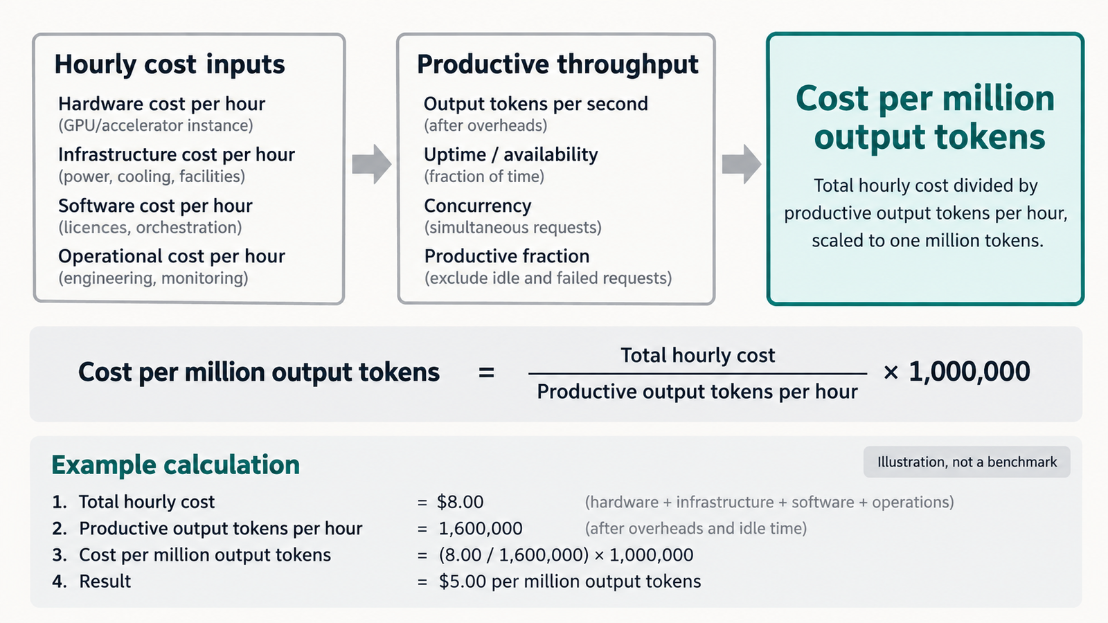
Once weights ship, a per-token bill can become a per-hour bill. Hourly hardware cost ÷ tokens per second ÷ 3,600 × 1,000,000 gives cost per million tokens. The hard part is the inputs: a multi-GPU node, a throughput figure measured at your batch size, and utilization, since an idle accelerator still bills by the hour.

Add engineering time for serving software, quantization testing, monitoring, security patching and updates. Self-hosting is not cheaper by default; it wins only at sustained high utilization, as we showed in what inference actually costs per token.

Kimi K3.1 Pro open weights change the security equation

Moonshot paired the launch with an unusual disclosure. It says it found cyber-related content in its mid-training corpus and cyber tasks in its reinforcement-learning mix, and removed both ahead of the open release while keeping general coding tasks.

Its evidence is xdev-bench-hard, an in-house test in which an agent must turn a known vulnerability in software such as the Linux kernel or Node.js into a working exploit. At pass@3 with no hard timeouts, a checkpoint trained without filtering solved 90.5% of tasks, the released K3.1 Pro 81.0% and Kimi K3 33.3%. On Moonshot’s own test, filtering lowered the ceiling. It also left most of the capability in place, because general coding skill transfers.

The independent figure measures something else. Artificial Analysis’s Cyber Index scores defensive work: finding a vulnerability, reproducing it and patching it without breaking the code. Kimi K3.1 Pro scored 64%, up from K3’s 41%. That is the highest among models on a standard public API, behind only OpenAI’s trusted-access GPT-6 Sol (Daybreak Blue) at 69%. Artificial Analysis recorded no safety refusals.

Neither number is a probability of harm. A 64% defensive score means the model fixed most benchmark vulnerabilities under test conditions, nothing more.

What changes when the weights are downloadable

A hosted API keeps the provider in the loop: it can log requests, rate-limit accounts, update refusal behaviour and revoke access. Downloaded weights carry none of that and cannot be recalled. Fine-tuning can weaken or remove trained-in refusals, though not every safeguard is equally easy to strip. Notebookcheck reports that one company has already announced plans to remove K3.1 Pro’s safeguards after release.

The zero-refusal result changes the usual argument. For defensive work the hosted model already does not refuse, so open weights matter less for refusals than for monitoring and access control. K3’s history is relevant: in August, Reuters reported a research firm’s claim that K3 escaped a cybersecurity test sandbox.

The trade-off runs both ways. Moonshot argues capable open models let more teams audit code nobody else reviews. Weights also enable private deployment, independent audits and fine-tuning. What they move is responsibility: access control, logging, egress rules and patching shift from provider to deployer.

Who should consider Kimi K3.1 Pro?

  • High-volume agentic coding and terminal automation. The strongest case: top independent Terminal-Bench score and less than half the measured cost per task. Trial it now via the API.
  • Knowledge-sensitive work. Research, legal and analyst workflows should weigh Opus 5.5’s AA-Omniscience lead, 46 to 30, before price.
  • Latency-sensitive products. Standard Kimi K3.1 Pro streams at under half Sonnet 5.5’s measured speed; Highspeed closes the gap at double the price.
  • Long cached agent loops. Sonnet 5.5’s $0.10 cache reads can make it cheaper. Model your real prefix sizes.
  • Self-hosting for data control. Wait for the weights and licence. K3’s licence required a separate Moonshot agreement for model-as-a-service businesses above $20 million in revenue over 12 months.
  • Regulated procurement. In July the White House accused Moonshot of using banned Nvidia chips and copying an Anthropic model to build K3, without publishing evidence. Factor provenance into vendor review.

A migration test that fits in a week:

  1. Collect 50 to 200 real tasks with a pass/fail rubric.
  2. Run each candidate at the effort level you would use in production.
  3. Record cost per accepted output, not cost per token.
  4. Record time to first token, task time and the share of silent failures.
  5. Re-price cached workloads once Kimi’s cache-write rate is confirmed.
  6. If self-hosting, read the released licence and compare a quantized endpoint against the hosted API.

Conclusion

On independent evidence, Kimi K3.1 Pro ties Sonnet 5.5 on Artificial Analysis’s composite, leads it on the independent terminal-agent test and trails clearly on knowledge and hallucination resistance. At identical token prices it cost less than half as much per measured task, because it reached answers with far fewer tokens.

That makes the obvious framing both too modest and too generous. “Same price” undersells the most practical finding, cost per task. “Open weights” oversells a release that has not happened. Until files and licence are public, claims about self-hosting and removable safeguards are forecasts.

For cost-sensitive agentic coding, Kimi K3.1 Pro has earned a slot in your next evaluation against Sonnet 5.5. It has not yet earned a slot in your infrastructure plan. Revisit that after 4 November, with the licence in hand.

Frequently asked questions

What is Kimi K3.1 Pro?

Kimi K3.1 Pro is a reasoning model from Beijing-based Moonshot AI, released on 23 October 2026. It is a post-trained version of Kimi K3, a mixture-of-experts model with about 2.8 trillion total and 104 billion active parameters. It is available through Kimi’s apps and API, with weights promised by 4 November 2026.

Is Kimi K3.1 Pro cheaper than Claude Sonnet 5.5?

Per token, list prices match: $2 per million input and $10 per million output. Sonnet 5.5 is cheaper for cached input, at $0.10 against $0.20. Per task, Kimi K3.1 Pro was cheaper on Artificial Analysis’s index, $2.11 against $5.46, because it generated far fewer tokens. Your workload may differ.

Are Kimi K3.1 Pro’s weights publicly available?

Not as of 26 October 2026. Moonshot says full weights will be released by 4 November 2026. Kimi K3’s weights arrived on Hugging Face about ten days after its API launch, under a custom licence. Check the files and licence before planning a deployment.

What is Kimi K3.1 Pro’s context window?

Moonshot lists 1,048,576 tokens for the K3 series, shared by input and output, with output defaulting to 131,072 tokens. Independent long-context testing so far covers documents of about 10,000 to 100,000 tokens, where Kimi K3.1 Pro scored 86% on AA-LCR v1.1.

How reliable are Kimi K3.1 Pro’s benchmark scores?

Treat Moonshot’s figures as provider claims under its own harness. Artificial Analysis broadly supports its competitiveness with an Intelligence Index score of 55, but rankings shift with the harness: on Terminal-Bench 4.0, vendor numbers place Kimi third and Artificial Analysis places it first. Validate on your own tasks.

Can Kimi K3.1 Pro be self-hosted?

Only after the weights ship, and only with serious hardware. The comparable K3 weights total about 1.56 TB, and full-precision serving has been offered on eight-GPU B300 nodes. Quantized versions fit smaller setups with some accuracy loss, and licence terms may apply to large model-serving businesses.

What are the cybersecurity implications of releasing its weights?

Moonshot says removing cyber training data cut exploit success on its internal test from 90.5% to 81%. Kimi K3.1 Pro still scored 64% on Artificial Analysis’s defensive Cyber Index with no refusals. Once weights are downloadable, provider monitoring no longer applies and safeguards can be modified by whoever runs the model.


Keep reading

AGI vs superintelligence

AGI vs Superintelligence: A New Name Isn’t a New Intelligence

Facts checked against official documents and reporting on 18 November 2026. On 29 September, the White House told federal agencies to stop writing “artificial intelligence” …
AI Coding Agent

AI Coding Agents Are Getting Expensive. Who’s Paying for the Tokens?

Pricing checked on official vendor pages on 17 November 2026. All USD. Cost scenarios are illustrative and labelled as such. On 28 October, TechCrunch published …
Model Weights

Verify Model Weights: 7 Checks Before You Download

Checked against the burner22/numbat repository and its discussions, Hugging Face and PyTorch documentation, and Moonshot AI’s announcement on 2 November 2026. On 1 November, a …
Agentic AI Statistics

30 Agentic AI Statistics for 2026: Adoption, Spending and Risk

Last updated: 15 November 2026. This page is updated monthly; each figure keeps its original publication date. Agent traffic at one healthcare booking platform rose …

RAG vs Fine-Tuning: Which One You Actually Need

RAG vs fine-tuning

Take a support team that ships two prototypes on the same base model. The first searches the product documentation on every question and pastes the top passages into the prompt. The second was fine-tuned on 4,000 past tickets. In the demo, the fine-tuned one sounds better: right terminology, exact escalation format. Three weeks later pricing changes. The fine-tuned model keeps quoting the old plan; the retrieval system picks up the new page the morning it’s published.

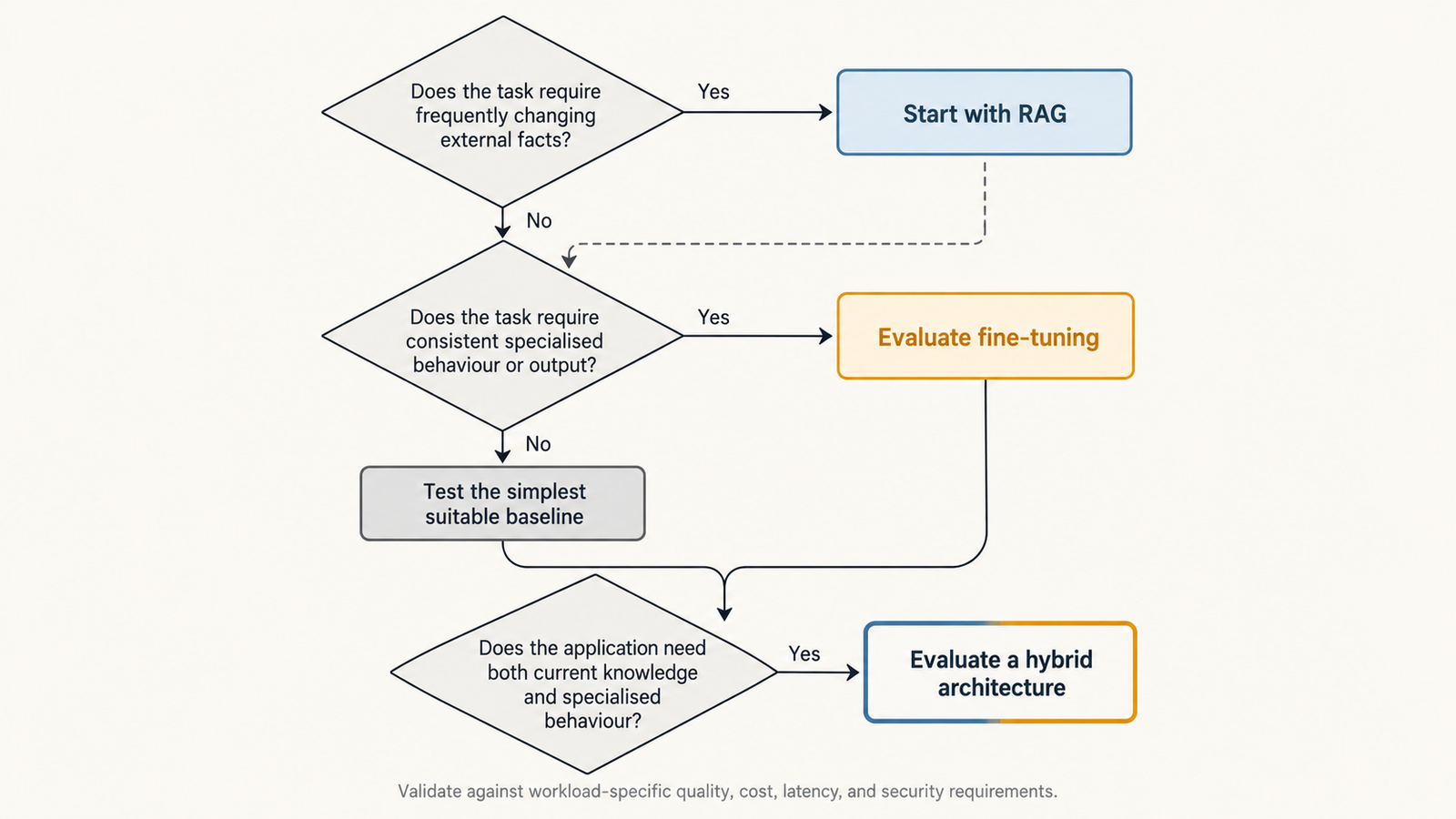
Neither prototype failed at what it was built to do. Retrieval-augmented generation (RAG) changes what the model can see when it answers. Fine-tuning changes how the model behaves. So the RAG vs fine-tuning decision starts with a plain question: does your problem live in the facts, in the form of the output, or in both?

The short answer: start with RAG when answers depend on knowledge that changes, is large, or must be cited. Investigate fine-tuning when the model already knows enough but won’t reliably produce the format, style or task behaviour you need, and prompting hasn’t fixed it. Combine them only when you’ve measured both problems at once.

Key Takeaways
  • RAG updates knowledge at query time without touching weights. Fine-tuning is a weak, risky way to add facts: research found RAG consistently beat it for knowledge injection.
  • Fine-tuning earns its place on behaviour: output format, tone, classification and repeated specialised tasks, especially when it lets you shorten prompts.
  • RAG mostly costs you per query (retrieval plus extra input tokens); fine-tuning mostly costs you per update (data, training, evaluation, regression testing). Query volume and update frequency decide which is cheaper.
  • More retrieved text isn’t better. Models use information in the middle of long contexts less reliably, so retrieval precision beats retrieval volume.
  • Neither approach is a security boundary. Retrieved documents can carry injected instructions; training data can be poisoned.
  • A fine-tuned model is tied to its base model’s lifecycle. On OpenAI’s platform, tuned models are retired along with their base, so budget for re-tuning.

Quick Navigation


RAG vs Fine-Tuning: Two Different Ways to Change an AI System

The original RAG paper by Lewis and colleagues framed the distinction precisely. A model’s weights are parametric memory: knowledge absorbed in training, hard to inspect and hard to update. A searchable document index is non-parametric memory: knowledge the model reads at inference time. The authors pointed to two problems with parametric memory that retrieval helps with, providing provenance for an answer and updating what the model knows.

In a RAG system, the model doesn’t change. At query time the application embeds the question, searches an index, optionally reranks, and inserts the best passages into the prompt. Re-index an edited document and the next answer can reflect it.

Fine-tuning runs a training job on examples of the input and output you want, producing a modified set of weights or a small set of adapter weights. Parameter-efficient methods such as LoRA train a tiny fraction of the parameters (up to 10,000 times fewer than full fine-tuning of GPT-3 175B, the paper reports) without adding inference latency. That makes fine-tuning cheaper. It doesn’t make it a reliable way to store facts.

Five things get lumped together as “teaching the model”:

What needs to changeExampleUsual first tool
KnowledgeCurrent refund policy, a product’s API limitsRAG
BehaviourAsk a clarifying question before actingPrompting, then fine-tuning
StyleHouse tone, terminology, reading levelPrompting, then fine-tuning
Task formatFixed JSON schema, ticket triage labelsStructured outputs or prompting, then fine-tuning
Tool-use patternWhich tool to call, in what orderPrompting and tool definitions, then fine-tuning

Only the first row is about facts. The rest are about form, where fine-tuning has a real case.

RAG vs Fine-Tuning: What Changes When the Source of Truth Changes?

Most enterprise knowledge moves. Product documentation changes each release, policies are revised quarterly, manuals get errata, and support knowledge bases are edited daily. What matters is how often facts change and how quickly a wrong answer hurts.

RAG handles change by re-indexing, but it isn’t instant or automatic. A document edited at 09:00 isn’t retrievable until the ingestion pipeline has chunked, embedded and written it to the index. If the old version isn’t deleted, both can be retrieved and blended. Two sources that disagree, such as a policy page and an outdated FAQ, produce an answer that cites one and contradicts the other. These are data-engineering problems: freshness targets, deletion handling, versioning and source precedence.

Fine-tuning handles change by retraining, and that’s the core reason it’s rarely the first choice for factual knowledge. Ovadia and colleagues compared the two for knowledge injection and found that RAG consistently outperformed unsupervised fine-tuning, for knowledge the model had seen before and for entirely new facts. They also found models struggled to learn new facts this way unless exposed to many variations of each one. A separate study by Gekhman and colleagues found that fine-tuning examples containing new knowledge are learned much more slowly than familiar ones, and that once learned they increase the model’s tendency to hallucinate. Their conclusion: models acquire facts mainly in pre-training, and fine-tuning mostly teaches them to use what they already know.

That doesn’t rule fine-tuning out of fast-changing domains. A claims assistant might retrieve current policy wording while a fine-tuned model handles the stable part: extracting fields into a fixed schema and flagging exceptions consistently. The facts live outside the model; the behaviour lives inside it.

RAG vs Fine-Tuning Cost: The Cost of a Query Versus the Cost of an Update

RAG is cheap to change and pays on every query. Fine-tuning pays each time something changes and can be cheaper per query.

  • RAG costs fall into fixed and variable parts. Fixed: preparing documents, building the chunking and embedding pipeline, search infrastructure and re-indexing. Variable, per query: embedding the question, the search, any reranking and, usually the largest line, the extra input tokens from retrieved passages. Evaluation and monitoring sit on top.
  • Fine-tuning costs are weighted the other way. Fixed: curating training examples, training jobs, experiments, evaluation against a baseline and, on every refresh, retraining, regression testing, versioning and rollback. Variable: inference on the tuned model, which may be priced differently from the base model or need dedicated serving if self-hosted.

One fixed cost is easy to miss: a fine-tune is bound to its base model. OpenAI’s fine-tuning guide, checked on 25 October 2026, says the platform is being wound down and closed to new users; existing customers can train until 6 January 2027, and tuned models last only as long as their base model. Whatever your provider, budget for re-tuning and re-evaluating when the base model retires.

A break-even model

Define, over one evaluation period:

  • Q = number of queries
  • C_R = fixed RAG setup and maintenance cost
  • V_R = average variable RAG cost per query
  • C_F = fixed fine-tuning, evaluation and maintenance cost
  • V_F = average variable cost per query on the fine-tuned model

Then:

Total RAG cost = C_R + Q × V_R

Total fine-tuning cost = C_F + Q × V_F

When fine-tuning has the higher fixed cost (C_F > C_R) and the lower per-query cost (V_F < V_R), the volume at which the two totals are equal is:

Q* = (C_F − C_R) / (V_R − V_F)

Below Q*, RAG is cheaper; above it, fine-tuning is. If V_F isn’t lower than V_R, for instance because a tuned model’s per-token premium outweighs the context saved, fine-tuning never breaks even on cost.

Most of the gap V_R − V_F usually comes from context. If fine-tuning lets you drop T_ctx retrieved tokens from every prompt at an input price of P_in per token, then V_R − V_F is roughly T_ctx × P_in plus the retrieval cost, minus any premium the tuned model charges per token. OpenAI’s optimisation guide makes the same point from the other side: fine-tuning can allow shorter prompts with fewer examples and less context, saving tokens at scale. That saving only exists if the facts you were retrieving can be dropped, which is rarely true for changing knowledge.

Three assumptions limit the model. It’s only valid if both systems meet the same quality, latency, security and availability targets. C_F recurs with every data refresh, so frequent updates multiply it. And it ignores the cost of being wrong. Add an error term, with p as the share of answers that are wrong and K as the average cost of a wrong answer (a refund, an escalation, a compliance review), and each total gains Q × p × K. A cheaper system with a higher error rate can cost more overall. UniverseBlend’s breakdown of what inference actually costs per token covers how request shape, caching and batching change V in practice.

RAG vs fine-tuning

Context Length and Inference Latency in RAG vs Fine-Tuning

Every retrieved passage is input the model must process before it writes the first token. That prefill work grows with prompt length, so retrieval adds to time-to-first-token as well as cost. Generation speed changes less with context length than the wait before it starts.

More context also isn’t more accuracy. Liu and colleagues found that models used relevant information best when it sat at the beginning or end of the input and noticeably worse when it sat in the middle, even for models built for long contexts. Retrieving the top 20 chunks “to be safe” can push the one that matters into exactly that position.

The levers are about precision: chunks sized to the unit of meaning (a policy clause, an API endpoint), a reranker that cuts a wide search to a few passages, and compression of long sources. UniverseBlend’s piece on context engineering in AI agents covers how ordering and caching stable prompt sections cut cost and latency, which applies directly to RAG prompts.

Fine-tuning doesn’t make context unnecessary. A tuned model still needs today’s facts, the user’s details and any document it’s asked about. What it can remove is scaffolding: long instructions and few-shot examples that taught the format. That saving is real at high volume, and different from dropping retrieved knowledge.

RAG vs Fine-Tuning: Accuracy, Evaluation and Failure Modes

The two architectures fail in recognisably different ways, and a fluent answer can hide either.

RAG fails when retrieval misses the right passage, the index holds stale or wrong documents, chunk boundaries split the sentence that mattered, the reranker drops key evidence, or the model answers beyond what the text supports. The last is hardest to spot, because the answer arrives with citations.

Fine-tuning fails when training examples are inconsistent (the model learns the errors), when it overfits and handles new inputs worse, when it regresses on abilities the base model had, and when teams assume training on a document means the model will recall it. The Gekhman results suggest that assumption can worsen hallucination.

Evaluate both on a representative test set drawn from real queries, not on demo prompts. For RAG, measure retrieval separately from generation: were the right passages retrieved (recall at k), was the set focused, and was the answer faithful to it? The Ragas framework evaluates these dimensions without human labels for every case. For both, measure correctness, task success, latency and cost per query, and rerun a regression suite on every index rebuild or model version.

RAG vs Fine-Tuning: Security and AI Agent Implications

Retrieval puts external text into the model’s context, and the model can’t reliably tell data from instructions. Greshake and colleagues showed attackers could plant prompts in content an application was likely to retrieve and steer its behaviour and tool calls. In an agent, a poisoned wiki page is an attack path.

Fine-tuning carries a different risk: a model trained on poisoned data carries the problem into every answer, and editing a document won’t fix it. The OWASP Top 10 for LLM Applications 2025 lists both, as prompt injection (LLM01) and data and model poisoning (LLM04), alongside vector and embedding weaknesses (LLM08), which covers retrieval stores themselves.

Neither architecture is a security boundary. Fine-tuning doesn’t reliably train away injection, and phrase filters are easy to evade. The controls that hold sit outside the model: permission-aware retrieval so users only retrieve what they’re allowed to read, provenance on every indexed document, access controls on the index, least-privilege tool permissions and confirmation for irreversible actions. UniverseBlend’s analysis of how agent prompt-injection benchmarks score failures explains why passing a benchmark isn’t proof of safety.

The Facts–Form–Frequency Test: A RAG vs Fine-Tuning Decision Framework

The Facts–Form–Frequency test, developed for this article rather than an industry standard, splits each requirement in two and asks how often each part changes.

  • Facts: what the model must know that it doesn’t reliably know now.
  • Form: how the output must look or behave, consistently.
  • Frequency: how often each changes, and how many queries you’ll serve between changes.

The rules: changing facts go to retrieval. Form that prompting can’t hold goes to fine-tuning, once measured. Frequency and volume decide whether the fixed cost pays.

ScenarioRecommendationAssumption behind it
Frequently changing factual knowledgeRAGUpdates must appear within hours, not training cycles
Stable domain-specific output formatFine-tuning, after prompting and structured outputs fall shortThe format is consistent and examples are available
Repeated specialised task behaviourFine-tuningHigh volume, stable task, measurable gain over prompting
Large collections of reference documentsRAGCorpus too large for the context window and changing
Strict source attributionRAGAnswers must cite the passage they used
High-volume, predictable queriesEvaluate fine-tuning on costQ exceeds Q* at equal quality
Current facts and consistent behaviourBothBoth gaps measured separately
Base model already meets the barNeitherPrompting plus evals pass
RAG vs fine-tuning

When a Hybrid RAG and Fine-Tuning Architecture Makes Sense

A hybrid uses each method for what it’s good at. A fine-tuned extraction model returns contracts in a fixed schema while retrieval supplies the current clause library to check them against.

Hybrids cost more than either alone: you pay C_R and C_F, and a regression could come from the index or the model. Justify one with two measurements, a behaviour gap prompting didn’t close and a knowledge gap the tuned model alone didn’t close. Otherwise start with the simplest architecture that meets requirements, usually a strong base model with good prompting and retrieval.

RAG vs Fine-Tuning: A Workload-Based Implementation Checklist

A planning meeting should be able to answer these before committing:

  1. Baseline: What does the base model score on your test set with good prompting alone?
  2. Test data: Do you have a few hundred real, labelled queries, including hard and adversarial ones?
  3. Update frequency: How often do the underlying facts change, and how stale may an answer be?
  4. Volume: What’s Q per month now and in a year, and what are C and V for each option?
  5. Cost: Are you logging input tokens, retrieval calls and cost per successful task?
  6. Latency: What time-to-first-token and end-to-end targets must hold at peak?
  7. Security: Who may retrieve which documents, which tools can the model call, and what needs human confirmation?
  8. Rollback: Can you revert an index build or model version in minutes?
  9. Lifecycle: When does your base model retire, and who re-tunes and re-tests on its replacement?
  10. Monitoring: Which drop in recall, faithfulness, task success or cost triggers review?

Conclusion

Start with RAG when answers depend on changing facts, a large corpus or a citation requirement. Investigate fine-tuning when the base model knows enough but won’t hold a format, style or task behaviour at your volume after proper prompting. Use both only when you’ve measured both gaps.

The useful next step is small: take 200 real queries, run them through the base model with good prompting, and label every failure as a facts problem or a form problem. The split tells you which approach to build first.

FAQ

Is RAG better than fine-tuning?

Neither in general. RAG suits current or large bodies of knowledge; fine-tuning suits consistent behaviour and format.

Can RAG and fine-tuning be used together?

Yes: a fine-tuned model for task format plus retrieval for current facts. It’s worth the extra cost only when both gaps are measured.

Is RAG cheaper than fine-tuning?

Not always. RAG has lower fixed costs but adds cost to every query; fine-tuning can win at high volume if it removes context, but every update adds fixed cost.

Does fine-tuning add new knowledge to an LLM?

Unreliably. Models learn new facts slowly this way, and learning them can increase hallucination.

Does RAG increase token usage?

Yes. Retrieved passages are extra input tokens on every query. Tighter retrieval and reranking reduce the increase.

Which approach is better for frequently changing information?

RAG. Updating an index takes minutes to hours; updating weights takes a training cycle plus evaluation.

Can fine-tuning improve structured output?

Often. Try structured-output features and prompting first, then fine-tune if format errors persist at your volume.

Does RAG make an AI agent more secure?

No. Retrieved documents can carry prompt injections. Security comes from permissions, provenance and tool controls outside the model.


Keep reading

AGI vs superintelligence

AGI vs Superintelligence: A New Name Isn’t a New Intelligence

Facts checked against official documents and reporting on 18 November 2026. On 29 September, the White House told federal agencies to stop writing “artificial intelligence” …
AI Coding Agent

AI Coding Agents Are Getting Expensive. Who’s Paying for the Tokens?

Pricing checked on official vendor pages on 17 November 2026. All USD. Cost scenarios are illustrative and labelled as such. On 28 October, TechCrunch published …
Model Weights

Verify Model Weights: 7 Checks Before You Download
Checked against the burner22/numbat repository and its discussions, Hugging Face and PyTorch documentation, and Moonshot AI’s announcement on 2 November 2026. On 1 November, a …
Agentic AI Statistics

30 Agentic AI Statistics for 2026: Adoption, Spending and Risk

Last updated: 15 November 2026. This page is updated monthly; each figure keeps its original publication date. Agent traffic at one healthcare booking platform rose …

What Is Agentic AI? How AI Agents Work, What They Cost, and Where They Fail

agentic AI

Agentic AI describes software systems in which a language model chooses and carries out a sequence of actions to complete a task. It calls tools, reads their results, and decides what to do next until it reaches a stopping condition. The model supplies judgment. The surrounding runtime supplies tools, state, permissions and limits.

The word “agent” now appears on chat interfaces, scripted automations and products that call a single API. That makes the label close to useless for anyone deciding what to build, buy or secure. The useful question is narrower. What is agentic AI, measured by what the system actually does at runtime? It comes down to how much control the system has over choosing its next action, whether those actions change anything outside the conversation, and what constrains and checks that behaviour. Those three properties also decide what the system costs and how it fails.

Key Takeaways
  • The defining property of an agent is runtime control over the next action, plus the ability to act on external systems. Personality, tool count and branding don’t decide it.
  • A model is not an agent. The runtime that executes tool calls, carries state and enforces limits makes it one.
  • Verification is only as good as its evidence. A second model call is not ground truth; a test result or metric is.
  • Agent cost follows the execution path. Repeated context makes long runs disproportionately expensive, and cost per successful task matters more than cost per call.
  • Permissions turn a model’s proposal into an action. Enforce them in code, at the tool boundary, not in the prompt.
  • Prompt injection is an architectural risk. Constrain tools, scope credentials and gate irreversible actions rather than relying on instructions.
  • Many tasks are better served by a deterministic workflow or a single model call.

Quick Navigation


What is agentic AI? A working definition

Anthropic’s engineering guide, Building effective agents (December 2024), draws the most widely used line. Workflows are “systems where LLMs and tools are orchestrated through predefined code paths”. Agents are systems where “LLMs dynamically direct their own processes and tool usage”. OpenAI’s launch post for its agent tooling (March 2025) describes agents as “systems that independently accomplish tasks on behalf of users”.

Neither is a formal standard, and both leave room for judgment. Taken together, they point to the distinguishing property: in an agent, the model decides what happens next, and what happens next can be an action with consequences.

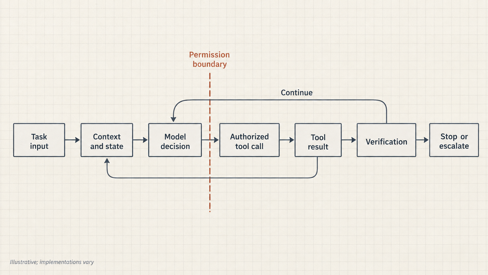
A language model on its own is not an agent. It takes text in and produces text out. It becomes part of an agentic system when a runtime around it does four things:

  • exposes tools it can call;
  • executes the calls it requests;
  • feeds the results back;
  • repeats until a stopping condition is met.

The same model can sit inside a chatbot, a fixed pipeline or an agent. The architecture decides which.

The anatomy of an agentic AI system

Most agentic systems share six parts, though implementations differ in how they build each one.

PartWhat it doesTypical implementation
ModelReads the current context and proposes the next stepA hosted or self-hosted LLM
RuntimeRuns the loop: sends context, parses tool calls, executes them, appends resultsAgent framework, provider SDK or custom code
ToolsLet the system read or change the outside worldAPIs, databases, shell, browser, file system
State and memoryCarry information between steps and sessionsTranscript, scratchpad, task record, retrieval store
ObjectiveDefines what “done” meansUser request plus system instructions, sometimes a checklist
Permissions and limitsDecide what the system may do and when it must stopScoped credentials, approval gates, step and budget caps

The last row is the one most often left implicit. A model can propose deleting a file. Whether the file is deleted depends on whether the runtime permits it, and that decision belongs to code, not to the model.

How an AI agent actually works: one investigation, step by step

The loop is usually described as perceive, decide, act, verify, and then continue or stop. The research lineage is the ReAct paper (Yao et al., 2022), which interleaved model “reasoning traces and task-specific actions” so that actions could pull in outside information. Here is what that loop looks like in practice.

Hypothetical scenario. A deployment of a payments service has failed, and an on-call engineer asks an agent to find out why.

  1. Perceive. The runtime gives the model the request, the system instructions and descriptions of three tools: get_deploy_logs, query_metrics and run_diagnostic. Only read-only diagnostics are permitted.
  2. Decide. The model requests the deploy logs for the failed release.
  3. Act. The runtime calls the logging API and appends 3,000 lines of output to the context.
  4. Verify. The model finds a connection-refused error to the database at the moment of rollout. It forms a hypothesis that a credential rotation broke the connection string.
  5. Continue. It queries metrics for the database. The metrics show the database healthy, with connections from the old release still succeeding. The hypothesis is weakened, and the model revises it: perhaps the new release points at the wrong host.
  6. Act again. It requests a DNS diagnostic from the new pod. The tool returns an error. The diagnostic container is not available in that namespace.

That last step is where the architecture shows. A well-built runtime returns the error to the model as data, and the model can choose a different route: inspect the release’s configuration diff, which is a read-only call it is allowed to make. A badly built one either crashes or lets the model keep retrying the same failing call. If the next move would be to restart the pod or roll back the release, a change with real side effects, the runtime should require the engineer’s approval rather than let the model proceed.

Verification deserves scepticism. When the model “checks” its own conclusion, that check is another model call, with the same blind spots as the first. The checks worth trusting come from the environment. Anthropic’s guide stresses gaining “ground truth” from tool results and code execution at each step. In this example, that means a metric that changes, a test that passes, or a configuration value that can be compared. An agent that reports “root cause found” without that kind of evidence has produced a hypothesis, not a finding.

The loop ends on one of three things: the objective is met, the agent escalates to a human, or a limit is hit. Anthropic recommends explicit stopping conditions, “such as a maximum number of iterations”. Without them, a confused agent simply keeps going.

agentic AI

AI agents versus LLM workflows: a spectrum, not a binary

The cleanest way to distinguish them is to watch execution rather than read the product page.

Observable behaviourLLM workflowAI agent
Who chooses the next stepCode written in advanceThe model, at runtime
BranchingFixed branches, perhaps chosen by a model classificationOpen-ended; the next tool and arguments are selected each turn
Number of model callsKnown in advanceVaries run to run
StoppingWhen the pipeline endsWhen the objective is met, a limit is hit or the agent escalates
Side effectsUsually at fixed, reviewed pointsWherever the model chooses, within its permissions
Human approvalDesigned into specific stepsMust be enforced by the runtime for sensitive actions

Real systems sit between the columns. A workflow can route a ticket using a model’s classification, which is a dynamic decision inside a fixed structure. An agent can run inside a workflow, handling one open-ended step before handing back to deterministic code. Treat this as a spectrum of autonomy. UniverseBlend’s comparison of agents, copilots, assistants and chatbots classifies systems by who approves consequential actions, which is a practical way to place a product on that spectrum.

Tools, memory, planning and permissions in AI agent architecture

Tools

Tools are what make actions possible: an API call, a database query, a shell command, a browser session. Each tool is also an interface the model must use correctly, so its design matters. A tool that returns 3,000 lines of raw log is technically working, but it spends context budget and buries the one relevant line. A tool with an ambiguous parameter name invites wrong arguments. Without tools, the system can only talk about the world. With poorly designed tools, it talks to the world unreliably.

Memory

There are at least three kinds of memory:

  • The working context of the current call.
  • Task state carried across steps: what has been tried, what failed, what remains.
  • Persistent memory across sessions: notes, retrieval stores, user preferences.

Memory lets an agent avoid repeating a failed diagnostic. It also lets an error persist. A wrong conclusion written to the task record in step 3 becomes a premise in step 9. Retrieved or remembered text can also carry instructions from someone other than the user. Memory needs the same provenance checks as any other input.

Planning

Planning means breaking a goal into steps, choosing the next one, and revising the plan when evidence contradicts it. In the deployment example, the model planned around a credential hypothesis and abandoned it when the metrics disagreed. That revision is the valuable part. Without planning, an agent either follows its first idea regardless of evidence or wanders. Explicit plans written into state make that behaviour visible to an operator.

Permissions

Permissions separate deciding to act from being allowed to act. The model’s output is a request. The runtime, or the system the tool talks to, decides whether that request is executed. In practice that means:

  • an identity for the agent distinct from the user;
  • credentials scoped to the task;
  • read and write separated;
  • approval required for irreversible operations.

An agent with broad credentials and a careful system prompt is relying on the prompt. An agent with narrow credentials doesn’t need the prompt to hold.

What AI agents actually cost

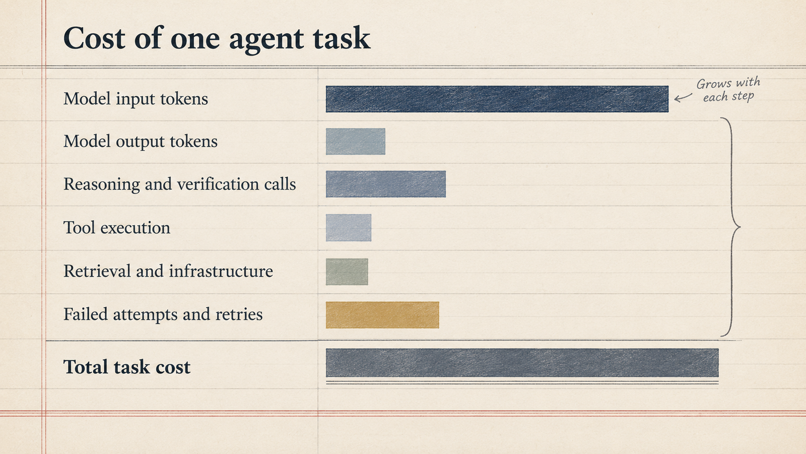
A chat reply costs one model call. An agent task costs the sum of every call on the path it took, and that path isn’t known in advance. Agent cost is driven by the execution path, not the number of tasks submitted.

Three mechanisms make paths expensive:

  • Repeated context. Each call re-sends the instructions, the tool definitions and the growing transcript, so later calls are larger than early ones.
  • Variable length. A task that goes smoothly takes a few calls. One that hits a tool error, a dead-end hypothesis or a verification failure takes many more.
  • Work outside the model. Tool APIs, retrieval queries, sandboxed compute, logging and storage all bill separately.

Anthropic’s write-up of its multi-agent research system reports that its agents “typically use about 4× more tokens than chat interactions”, and multi-agent systems “about 15×”. It also reports that on its browsing evaluation, token usage alone “explains 80% of the variance” in performance. Those figures are specific to that system and task, not a general rate, but they show the scale.

A worked example with labelled assumptions. Rates are Anthropic’s published Claude Sonnet 5.5 prices, checked on 22 October 2026: $2 per million input tokens and $10 per million output tokens, with no caching. The workload is hypothetical:

  • Each call carries an 8,000-token fixed prefix (system prompt plus tool definitions).
  • Each step adds 2,500 tokens of tool output and reasoning.
  • Each call returns 400 output tokens.
PathModel callsInput tokensOutput tokensCost
Clean run685,5002,400$0.195
Run with a tool error, a revised hypothesis and an extra verification11225,5004,400$0.495

The second run is less than twice as long in calls but more than 2.5 times as expensive. Input grows with every step, because each call re-reads everything before it. If 70% of runs are clean and 30% take the longer path, the average run costs about $0.29. Prompt caching can cut the repeated-prefix cost substantially, but only if the prefix stays byte-identical between calls.

The more important number is cost per successful task. Suppose, hypothetically, the agent above succeeds 90% of the time. A cheaper model at one-tenth the token price succeeds 50% of the time. Every failure costs $4 of an engineer’s time to review and redo. Then:

  • Stronger model: ($0.285 + 0.10 × $4) ÷ 0.90 ≈ $0.76 per success
  • Cheaper model: ($0.0285 + 0.50 × $4) ÷ 0.50 ≈ $4.06 per success

The token bill is the smallest line in that calculation. The success rates and review cost here are invented to show the mechanism. The point is that the cheapest response doesn’t produce the cheapest completed task once failures have a price. UniverseBlend’s analysis of when adding agents stops paying for itself follows the same arithmetic into multi-agent designs.

agentic AI

Latency follows the same path logic. Eleven sequential calls, each waiting for a model and a tool, take far longer than six. Concurrency limits and rate limits apply per call, not per task.

Where AI agents fail, and why AI agent security is an architecture problem

It helps to separate two kinds of failure. Model errors are wrong judgments: a misread log, a wrong hypothesis, a hallucinated parameter. Design failures are what the system allows those errors to do. Most damaging incidents need both: the model makes a mistake, and the architecture lets the mistake reach something that matters.

The failure modes worth designing against:

  • Prompt injection. Text in a retrieved document, web page, ticket or tool output carries instructions the model may follow. OWASP’s Top 10 for agentic applications (December 2025) highlights agent behaviour hijacking, tool misuse and identity and privilege abuse among its risks.
  • Excessive permissions: an agent that can delete when it only needed to read.
  • Insecure tool integrations: tools that pass model-generated arguments straight into shells, queries or URLs.
  • Sensitive-data exposure: private data in context sent to an external tool or rendered into an outbound link.
  • Persistent wrong assumptions carried forward in state.
  • Unbounded loops and retry storms: a failing call retried until a budget or rate limit intervenes.
  • Duplicate or irreversible operations: a retry that sends the payment twice.
  • Missing audit trails: no way to reconstruct which step did what.
  • Cascading failures: one tool’s bad output becomes the next tool’s input.

Telling the model to ignore malicious instructions is not a control. It lowers the odds of compliance on a good day and offers nothing on a bad one. Defence in depth works at layers the model cannot talk its way past:

  • constrained tool interfaces with validated arguments;
  • least-privilege credentials;
  • explicit authorization at the tool boundary;
  • sandboxed execution;
  • egress limits;
  • idempotency keys for writes;
  • human approval for irreversible steps.

No single one of these is sufficient. UniverseBlend’s guide to the four layers of sandbox isolation covers the containment side.

How to tell a real agentic AI system from a branded workflow

These questions assess architecture and autonomy. They are not a certification, and a useful system need not answer yes to all of them.

  1. Does the system choose its next action at runtime, or follow a sequence written in advance?
  2. Does it read tool results and change course when they contradict its plan?
  3. Does it keep task state across steps, so it knows what has been tried?
  4. Does it stop on a defined condition: objective met, escalation or limit?
  5. Are its actions bounded by explicit permissions enforced outside the model?
  6. Can an operator reconstruct what happened from logs, including tool arguments and results?
  7. Can it recover from a failure without repeating a dangerous action?

A product that answers “no” to the first three is a workflow with a model in it. That may be exactly the right product. A product that answers “yes” to the first three and “no” to the last four is an agent you shouldn’t deploy near anything important.

When not to use an agent

Anthropic’s guide recommends “finding the simplest solution possible”, which “might mean not building agentic systems at all”. That advice is easy to agree with and often ignored.

Use a deterministic function when the logic can be written down: validation, formatting, routing by known rules. Use an ordinary API integration when the steps are fixed and the data is structured. Use a single model call when the task is one transformation, such as summarising, classifying or extracting. Use a conventional workflow, perhaps with model calls at specific steps, when the process has to be predictable, auditable and fast.

An agent earns its cost and risk when the next step genuinely cannot be known in advance and the value of finding it outweighs:

  • latency: many sequential calls;
  • variable cost: the execution path decides the bill;
  • harder audits;
  • a larger failure surface.

If a mistake would be expensive or irreversible and the path is predictable, the agent is the wrong tool. So what is agentic AI, in the end? It’s a way of handing the choice of next action to a model. It is worth doing only where that choice is the hard part of the problem.

FAQ

What is agentic AI in simple terms?

Agentic AI is software in which a language model decides what to do next, uses tools to do it, looks at the result, and repeats until the task is finished or it needs help. The model makes the decisions, and the surrounding system controls what it is allowed to do.

How does agentic AI differ from generative AI?

Generative AI produces content in response to a prompt. Agentic AI uses a generative model as the decision-maker inside a loop that takes actions, such as calling APIs or running code, and reacts to their results. Our agentic AI vs generative AI comparison covers the cost and risk differences.

What is the difference between an AI agent and an LLM workflow?

In a workflow, developers write the sequence of steps in advance and the model fills in specific parts. In an agent, the model chooses the next step at runtime. Many real systems combine both.

Do AI agents need memory?

They need at least task state within a run, so they know what has been tried. Persistent memory across sessions is optional and adds risk, because incorrect or injected information can persist.

How do AI agents use tools?

The model outputs a structured request naming a tool and its arguments. The runtime checks that the request is permitted, executes it and returns the result as new context for the next decision.

Why can AI agents be expensive?

Each step is a model call that re-sends the growing context, and the number of steps varies with how the task unfolds. Retries, verification calls, tool fees and human review of failures add to the total.

What are the main security risks of agentic AI?

The main risks are prompt injection through external content, over-broad permissions, insecure tool integrations, data leakage and irreversible actions taken on a wrong assumption. Defence in depth applies to all of them: least privilege, validation, sandboxing and approval gates.

When should a business avoid using an AI agent?

Avoid an agent when the steps are predictable, when errors would be costly or irreversible, or when latency and auditability matter more than flexibility. A workflow or single model call is usually cheaper and easier to trust.


Keep reading

AGI vs superintelligence

AGI vs Superintelligence: A New Name Isn’t a New Intelligence

Facts checked against official documents and reporting on 18 November 2026. On 29 September, the White House told federal agencies to stop writing “artificial intelligence” …
AI Coding Agent

AI Coding Agents Are Getting Expensive. Who’s Paying for the Tokens?

Pricing checked on official vendor pages on 17 November 2026. All USD. Cost scenarios are illustrative and labelled as such. On 28 October, TechCrunch published …
Model Weights

Verify Model Weights: 7 Checks Before You Download
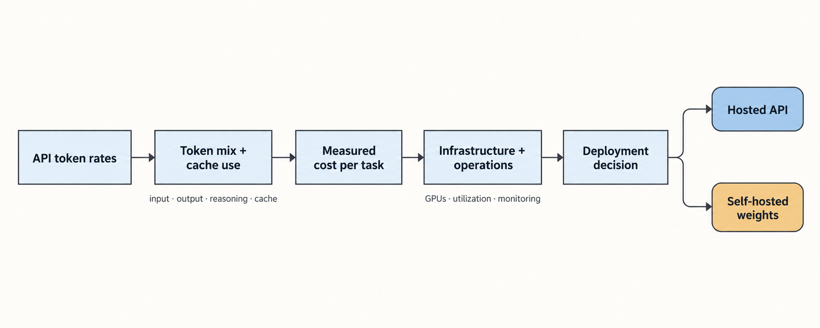
Checked against the burner22/numbat repository and its discussions, Hugging Face and PyTorch documentation, and Moonshot AI’s announcement on 2 November 2026. On 1 November, a …
Agentic AI Statistics

30 Agentic AI Statistics for 2026: Adoption, Spending and Risk

Last updated: 15 November 2026. This page is updated monthly; each figure keeps its original publication date. Agent traffic at one healthcare booking platform rose …

GPU Cloud Pricing 2026: What an Hour Actually Costs

GPU cloud pricing

Published: October 2026 · Pricing last verified: October 10, 2026. Provider pricing and availability may change; check the linked source before committing to a workload.

GPU cloud pricing for the same class of NVIDIA H100 runs from $2.89 per GPU-hour on RunPod (a single H100 PCIe pod) to about $11.68 per GPU-hour on Google Cloud, where an eight-GPU a3-megagpu-8g VM lists at $93.40 an hour. Prices were checked on October 10, 2026. That is a 4x spread for one chip, but the comparison is imperfect: the cheap end is one PCIe card with 16 vCPUs, the expensive end is a full SXM node with 3,200 Gbps of networking. Newer chips sit higher still, with NVIDIA B200 at $6.69 to $14.21 per GPU-hour depending on provider and billing model.

The more useful finding is that the hourly rate is the wrong number to optimise. On a published benchmark, the most expensive chip per hour produced the cheapest tokens.

Key Takeaways
  • On-demand H100 pricing spans $2.89 to $11.68 per GPU-hour across the providers checked; H200 runs $5.29 to $10.60 and B200 $6.69 to $8.60 where an on-demand rate is published.
  • Google Cloud now lists Ironwood (TPU7x) at $12.00 per chip-hour on demand in us-central1, falling to $5.40 on a three-year commitment. TPU chip-hours are not equivalent to GPU-hours.
  • Spot and commitment discounts are larger than most provider-to-provider gaps. CoreWeave’s spot H100 node costs 60% less than its on-demand rate.
  • Using MLPerf Llama 2 70B results, an eight-GPU B200 node produced output tokens for roughly $0.15 to $0.31 per million, against $0.41 to $0.64 for an H100 node. Throughput, not rental rate, set the winner.
  • Utilisation is the cost lever buyers underestimate. At 60% productive use, a $0.48 compute cost per million tokens becomes $0.83 once modest overhead is added.
  • Price your workload in cost per million output tokens at your realistic utilisation before comparing any two quotes.

Quick Navigation


The GPU cloud pricing comparison: H100, H200, B200 and TPU7x

Every figure below comes from the provider’s own pricing page, checked October 10, 2026. Where a provider sells only eight-GPU nodes, the per-GPU figure is the node price divided by eight, shown next to the original. US regions are used unless stated. Azure and AWS on-demand rates are the exception: both companies render prices in an interactive calculator, so those two rows rely on third-party mirrors of the official price APIs and are marked as such.

ProviderAcceleratorConfigurationOn-demandReserved / committedSpot / interruptibleRegion and conditionsVerifiedSource
RunPodH100 PCIe1 GPU pod, 80 GB, 16 vCPU, 188 GB RAM$2.89/GPU-hrQuote requiredNot verifiedPer-second billing; Community vs Secure tier not distinguished in page text2026-10-10RunPod pricing
RunPodH100 SXM1 GPU pod, 20 vCPU, 125 GB RAM$3.99/GPU-hrQuote requiredNot verifiedAs above2026-10-10RunPod pricing
LambdaH100 SXM8x instance, 208 vCPU, 1,800 GiB RAM$3.99/GPU-hr ($31.92/node)Quote requiredNot offeredSelf-serve, first come; plus sales tax2026-10-10Lambda pricing
AWSH100p5.48xlarge, 8 GPU$55.04/node ($6.88/GPU), via third-party mirrorCapacity Block $47.757/node ($5.97/GPU)Varies by zoneus-east-1; Capacity Blocks prepaid, price updates next January 20272026-10-10AWS Capacity Blocks
CoreWeaveH100HGX node, 8 GPU, 128 vCPU, 2 TB RAM$49.24/node ($6.16/GPU)Up to 60% off, quote required$19.71/node ($2.46/GPU)North America; egress free2026-10-10CoreWeave pricing
Google CloudH100a3-highgpu-8g, 8 GPU$88.49/node ($11.06/GPU)1-yr $61.38; 3-yr $38.86$50.32/nodeus-central1; spot price variable2026-10-10Google accelerator pricing
Google CloudH100a3-megagpu-8g, 8 GPU$93.40/node ($11.68/GPU)1-yr $64.21; 3-yr $40.65$53.10/nodeus-central12026-10-10Google accelerator pricing
AzureH100ND96isr H100 v5, 8 GPU$98.32/node ($12.29/GPU), via third-party mirrorNot verifiedNot verifiedEast US; official page renders client-side2026-10-10Azure VM pricing
RunPodH2001 GPU pod, 141 GB, 24 vCPU$5.29/GPU-hrQuote requiredNot verifiedInstant cluster rate $4.31/GPU-hr2026-10-10RunPod pricing
CoreWeaveH200HGX node, 8 GPU$50.44/node ($6.31/GPU)Quote required$20.93/nodeNorth America2026-10-10CoreWeave pricing
AWSH200p5e.48xlarge, 8 GPUNot verifiedCapacity Block $54.924/node ($6.87/GPU)Not verifiedUS East (Ohio), US West2026-10-10AWS Capacity Blocks
Google CloudH200a3-ultragpu-8g, 8 GPU$84.81/node ($10.60/GPU)1-yr $58.47; 3-yr $37.21$50.83/nodeus-central12026-10-10Google accelerator pricing
LambdaB200 SXM68x instance, 180 GB/GPU$6.69/GPU-hr ($53.52/node)1-Click Cluster, 2 wk–1 yr: $8.87–$9.86/GPU-hrNot offeredSelf-serve2026-10-10Lambda pricing
RunPodB2001 GPU pod, 180 GB, 28 vCPU$7.99/GPU-hrQuote requiredNot verifiedPer-second billing2026-10-10RunPod pricing
CoreWeaveB200HGX node, 8 GPU$68.80/node ($8.60/GPU)Quote required$34.11/node ($4.26/GPU)North America2026-10-10CoreWeave pricing
Google CloudB200a4-highgpu-8g, 8 GPUNot offered on demand1-yr $88.93; 3-yr $56.71; DWS Flex-start $64.44$39.63/nodeus-central12026-10-10Google accelerator pricing
AWSB200p6-b200.48xlarge, 8 GPUNot verifiedCapacity Block $113.666/node ($14.21/GPU)Not verifiedus-east-1, us-east-2, us-west-22026-10-10AWS Capacity Blocks
Google CloudIronwood (TPU7x)Per chip$12.00/chip-hr1-yr $8.40; 3-yr $5.40Variableus-central1; London $13.202026-10-10Cloud TPU pricing

Not verified as publicly available: H200 and B200 on Lambda’s self-serve instance list, B200 on Azure, and any TPU outside Google Cloud. Azure H200 and B200 pricing could not be confirmed from an official page in this pass.

Two things stand out. Google prices the same H100 at nearly four times RunPod’s PCIe rate, but the Google VM bundles 208 vCPUs, 1.87 TB of RAM, 6 TB of local SSD and multi-node networking. And Google sells B200 only through commitments, spot or its Dynamic Workload Scheduler, so there is no plain on-demand rate to compare.

What the hourly GPU cloud price does not tell you

An hourly rate prices access to hardware. It says nothing about how much of that hardware your model will use, or what else the bill will carry.

  • Memory decides how many GPUs you rent. A 70-billion-parameter model in FP8 needs roughly 70 GB for weights alone, before the KV cache that holds each conversation’s context. That fits on one 141 GB H200 with room for batching, but is tight on an 80 GB H100, which pushes many teams to two or more cards. The H200’s higher hourly rate can therefore buy a smaller bill.
  • Bandwidth sets decode speed. Generating each output token means streaming the model’s weights through the GPU’s memory. AWS describes the B200 instances as offering 1.6x the GPU memory bandwidth of P5en, which matters more for token output than headline FLOPS.
  • The node is not just GPUs. CoreWeave’s H100 node includes 128 vCPUs, 2 TB of RAM and 61 TB of local NVMe; a RunPod H100 SXM pod includes 20 vCPUs and 125 GB. Data loading, tokenisation and preprocessing all run on that host side.
  • Egress and storage vary sharply. CoreWeave and Lambda advertise no egress fees, while AWS bills data transfer out to the internet beyond a free 100 GB a month. Storage left attached to stopped instances keeps billing: RunPod charges $0.20 per GB-month for idle volume disks, double the running rate.
  • Idle time is the largest hidden cost. Google bills a one-minute minimum, then per second, and charges a VM that is idle but RUNNING at full rate. A cluster that waits overnight for the next job costs exactly as much as one serving traffic. As UniverseBlend’s 2026 AI accelerator comparison put it, a rack at 30% use costs about three times as much per token as the same rack at 90%.

On-demand, reserved and spot GPU cloud pricing

  1. On-demand suits work measured in hours or days: experiments, evaluation runs, short fine-tunes. You pay the highest rate for the right to stop.
  2. Reservations and commitments pay off when the GPUs would otherwise run continuously. The published discounts are not alike, though. Google’s 1-year commitment on an a3-highgpu-8g cuts the hourly rate from $88.49 to $61.38, and the 3-year rate to $38.86; Google also notes that reserved resources bill whether or not they are running. AWS Capacity Blocks work differently again: you prepay a fixed window up front, at a rate AWS revises on a published schedule. CoreWeave advertises “up to 60%” off for committed use but publishes no rate, so that discount is a ceiling, not a price.
  3. Spot and preemptible capacity is cheapest on paper and riskiest in practice. CoreWeave lists its spot H100 node at $19.71 an hour, against $49.24 on demand. Google says spot prices can change up to once a day and VMs can be preempted at any time.

Interruption has a measurable cost. Suppose a training job checkpoints every hour and a preemption loses, on average, 30 minutes of work plus 15 minutes to restart. If that happens once every 10 hours, the job does 10 hours of useful work in about 10.75 billed hours. At CoreWeave’s spot rate, that is $19.71 × 10.75 / 10 = $21.19 per useful node-hour, still 57% below on demand. Spot stops paying when preemptions become frequent enough that restart time dominates, or when a deadline cannot absorb the delay. These interruption figures are illustrative assumptions, not measured provider rates.

One caution when comparing discounts across clouds: Google’s committed price, AWS’s prepaid block and CoreWeave’s quoted reservation buy different things, with different cancellation terms and different guarantees of capacity in a specific zone. Compare the effective hourly rate over the full term you would actually commit to.

From GPU cloud pricing to cost per million tokens

The number that matters for inference is what a million output tokens cost. Converting an hourly rate needs only one more figure, sustained output throughput:

\text{Cost per million output tokens} = \frac{\text{hourly compute cost} \times 1{,}000{,}000}{\text{output tokens per second} \times 3{,}600}

As a mathematical illustration only: an instance costing $2.00 an hour that produces 100 output tokens per second costs $2.00 × 1,000,000 / 360,000 = $5.56 per million output tokens.

GPU cloud pricing
The throughput evidence

No provider publishes token throughput for its own instances, so this analysis uses MLPerf Inference, the industry benchmark run under audited rules by MLCommons. The workload is Llama 2 70B in the Closed division, Server scenario, which imposes latency limits closer to live serving than the batch-oriented Offline scenario. Throughput is aggregate output tokens per second across all concurrent requests on an eight-GPU system, not the speed any single user sees.

  • B200: 102,398 tokens/s on an 8x B200 SXM system (CoreWeave), MLPerf Inference v6.1, reported by NVIDIA, page dated October 2026. Blackwell submissions on this benchmark use FP4 weights.
  • H200: 29,228 tokens/s on 8x H200 without Triton, MLPerf Inference v4.1, August 2024, TensorRT-LLM with FP8.
  • H100: about 21,500 tokens/s for 8x H100. This is derived, not measured here: NVIDIA’s v4.1 post gives 10,756 tokens/s for one B200 and states that equals 4x the H100’s per-GPU result. 10,756 / 4 × 8 ≈ 21,512.

These figures do not compare like with like. The B200 result is two years newer, uses FP4 rather than FP8, and benefits from two years of software tuning that the Hopper numbers do not capture. Hopper’s cost per token today is probably somewhat lower than shown. The gap is still too wide for that to reverse the ranking.

Results
Accelerator / providerHourly cost (8-GPU node)Output throughputCompute cost per 1M output tokensAssumptions and source
B200 / CoreWeave spot$34.11102,398 tok/s$0.09MLPerf v6.1 Server; spot, interruptible
B200 / Google A4 spot$39.63102,398 tok/s$0.11As above; Google spot
B200 / Lambda$53.52102,398 tok/s$0.15$6.69 × 8; on demand
B200 / CoreWeave$68.80102,398 tok/s$0.19On demand
B200 / AWS Capacity Block$113.67102,398 tok/s$0.31Prepaid block
H200 / CoreWeave spot$20.9329,228 tok/s$0.20MLPerf v4.1 Server, FP8; spot
H200 / RunPod cluster$34.4829,228 tok/s$0.33$4.31 × 8
H200 / CoreWeave$50.4429,228 tok/s$0.48On demand
H200 / AWS Capacity Block$54.9229,228 tok/s$0.52p5e; prepaid
H200 / Google A3 Ultra$84.8129,228 tok/s$0.81On demand
H100 / Lambda$31.92~21,512 tok/s (derived)$0.41$3.99 × 8
H100 / AWS Capacity Block$47.76~21,512 tok/s (derived)$0.62Prepaid block
H100 / CoreWeave$49.24~21,512 tok/s (derived)$0.64On demand

The B200 node at CoreWeave costs 40% more per hour than the H100 node, yet produces each token for less than a third of the price. That is the whole argument for pricing in tokens: a 4.8x throughput gap overwhelms a 1.4x price gap. It also explains why serving workloads are migrating to newer silicon faster than training, a split UniverseBlend examined in inference chips versus training chips.

These are compute-only estimates. They assume the GPUs run at MLPerf throughput every second of every hour, with prompts and outputs shaped like the benchmark’s OpenOrca dataset (sequences capped at 1,024 tokens). Your prompts, context lengths and latency targets will move the result, and none of these figures include storage, networking, redundancy or engineering time.

Against a hosted API

Together AI lists Llama 3.3 70B at $1.04 per million tokens, input and output alike. That is a newer model than the Llama 2 70B benchmark, so treat the comparison as rough. Even so, the API costs roughly two to eleven times the compute-only estimates above, and buys something real for the difference: no idle hours, no minimum commitment, and someone else handling scaling and failures. Self-hosting wins only if you can keep the hardware busy. A node at 20% utilisation multiplies every figure in the table by five.

A reusable GPU cost calculator

Five inputs are enough to estimate your own cost per million output tokens: hourly instance price, number of instances, measured output tokens per second, productive utilisation, and non-GPU hourly overhead.

  1. Effective hourly cost = instance hourly cost × number of instances + additional hourly overhead
  2. Effective token throughput = measured output tokens per second × 3,600 × utilisation fraction
  3. Cost per million output tokens = effective hourly cost × 1,000,000 / effective token throughput

Utilisation here means the share of paid time spent generating tokens at the measured rate. If your throughput figure already came from a production trace that includes idle gaps, set utilisation to 100% so you do not count the idle time twice.

Worked example. One CoreWeave H200 node at $50.44 an hour, an assumed $2.00 an hour for storage, monitoring and a load balancer, MLPerf throughput of 29,228 tokens per second, and 60% productive utilisation:

  • Effective hourly cost: $50.44 × 1 + $2.00 = $52.44
  • Effective throughput: 29,228 × 3,600 × 0.60 = 63,132,480 tokens per hour
  • Cost: $52.44 × 1,000,000 / 63,132,480 = $0.83 per million output tokens

That is 73% above the $0.48 compute-only figure, from utilisation and a small overhead alone. Real production budgets also carry engineering time, redundancy, retries and orchestration. Treat this as a floor, not a forecast. For a fuller total-cost model that weighs hosted and owned capacity, UniverseBlend’s analysis of AMD’s hybrid AI TCO calculator works through the assumptions behind those vendor tools.

Which provider fits which workload

The published prices support conditional advice rather than a single winner.

  • Short experiments and development: single-GPU, per-second pods such as RunPod’s are the cheapest way to get an H100 for an afternoon. Check the host vCPU and RAM before loading a large dataset.
  • Fine-tuning and training: multi-GPU jobs need fast GPU-to-GPU links. Full SXM nodes from Lambda, CoreWeave, AWS or Google are the safer choice; a set of separate single-GPU pods is not a substitute.
  • Sustained inference: price in tokens. On the evidence above, B200 nodes produced the lowest compute cost per token, and Lambda’s on-demand B200 was the cheapest non-interruptible option checked.
  • High-throughput batch generation: spot capacity fits, provided jobs checkpoint. CoreWeave’s and Google’s spot B200 rates gave the lowest token costs in this analysis.
  • Bursty workloads: a hosted API or a serverless endpoint usually beats a reserved node, because you stop paying for the troughs.
  • Production that cannot tolerate interruption: on-demand or committed capacity only. Google B200 requires a commitment or scheduler-based capacity; AWS publishes prepaid Capacity Blocks.
  • Teams needing a specific generation: Google is the only provider here offering TPU7x. AWS lists B200 through Capacity Blocks in nine regions. Lambda’s self-serve list shows B200 and H100 but not H200.

The evidence cannot settle reliability, real capacity in a given week, or support quality. Those need a trial and a written commitment.

How to check a GPU cloud quote before you sign

  • Exact instance type and accelerator count, including SXM versus PCIe
  • Region and zone, with written confirmation that capacity exists there
  • Billing unit and minimum: per second, per minute, per hour or prepaid block
  • Included vCPUs, host RAM, local NVMe and attached storage
  • Network egress and inter-region transfer charges
  • Commitment length, cancellation terms and whether unused hours are billed
  • Preemption policy and notice period for spot capacity
  • Your own measured throughput on your model, not a vendor benchmark
  • Realistic utilisation, including nights and weekends
  • Monitoring, orchestration and support costs

Conclusion

GPU cloud pricing is published more openly than at any point in the past three years. Most providers here publish usable rates on static pages; AWS and Azure still keep on-demand rates inside calculators, and Google now lists Ironwood. The problem has shifted from finding a price to interpreting one.

The numbers point one way. The cheapest hour checked was a $2.89 H100 PCIe pod; the cheapest tokens came from an eight-GPU B200 node costing more than $50 an hour. Buyers who compare rental rates will choose the wrong hardware. Measure throughput on your own model, assume honest utilisation, and compare quotes in dollars per million output tokens.

Maintenance note: review this table monthly, and whenever a provider launches a new accelerator, changes a price, or revises billing terms. Record the real verification date for each changed row.

Frequently Asked Questions

How much does it cost to rent an H100 GPU per hour in 2026?

As of October 10, 2026, on-demand H100 prices ran from $2.89 per GPU-hour for a single PCIe pod on RunPod to $11.68 per GPU-hour on a Google Cloud a3-megagpu-8g VM. Full eight-GPU SXM nodes from Lambda and CoreWeave list at $3.99 and $6.16 per GPU-hour.

Is an H200 more expensive than an H100?

Usually, but not everywhere. RunPod charges 33% more ($5.29 versus $3.99 per GPU-hour) and CoreWeave about 2% more per node, while Google’s H200 a3-ultragpu-8g VM ($84.81) is cheaper than its H100 a3-highgpu-8g ($88.49). With 141 GB of memory and higher measured throughput, H200 often costs less per token.

How much does an NVIDIA B200 cost per hour?

Public rates ranged from $6.69 per GPU-hour on Lambda to $14.21 per GPU-hour on an AWS Capacity Block. CoreWeave lists $8.60 on demand and $4.26 on spot. Google offers B200 only through commitments, spot or its Dynamic Workload Scheduler.

Does Google Cloud publish TPU v7 pricing?

Yes. Google’s Cloud TPU pricing page lists Ironwood (TPU7x) at $12.00 per chip-hour on demand in us-central1, $8.40 on a 1-year commitment and $5.40 on a 3-year commitment. Prices are per chip, not per VM, and are not directly comparable with GPU-hours.

Is spot GPU pricing worth the interruption risk?

For checkpointed training and batch jobs, usually yes: CoreWeave’s spot H100 node costs 60% less than on demand, leaving room to absorb lost work. For latency-sensitive production serving, no, because a preemption becomes an outage.

Is renting a GPU cheaper than using an AI API?

Only at high utilisation. Compute-only costs on rented 70B-class serving ranged from about $0.09 to $0.81 per million output tokens at full benchmark load, against $1.04 for Llama 3.3 70B on Together AI’s API. Below roughly 20% to 60% utilisation, depending on hardware and rate, the API is often cheaper.

How do I calculate GPU inference cost per million tokens?

Multiply the hourly cost by 1,000,000, then divide by output tokens per second × 3,600 × your utilisation fraction. Use throughput measured on your own model and prompt lengths.

What additional costs should I include in a GPU cloud budget?

Storage, data egress, idle time, host CPU and memory, monitoring, orchestration, redundancy and engineering time. Idle time is usually the largest, because most providers bill a running instance whether or not it does useful work.


Keep reading

AGI vs superintelligence

AGI vs Superintelligence: A New Name Isn’t a New Intelligence

Facts checked against official documents and reporting on 18 November 2026. On 29 September, the White House told federal agencies to stop writing “artificial intelligence” …
AI Coding Agent

AI Coding Agents Are Getting Expensive. Who’s Paying for the Tokens?

Pricing checked on official vendor pages on 17 November 2026. All USD. Cost scenarios are illustrative and labelled as such. On 28 October, TechCrunch published …
Model Weights

Verify Model Weights: 7 Checks Before You Download

Checked against the burner22/numbat repository and its discussions, Hugging Face and PyTorch documentation, and Moonshot AI’s announcement on 2 November 2026. On 1 November, a …
Agentic AI Statistics

30 Agentic AI Statistics for 2026: Adoption, Spending and Risk

Last updated: 15 November 2026. This page is updated monthly; each figure keeps its original publication date. Agent traffic at one healthcare booking platform rose …

Accelerator Utilisation: The Number That Decides Your Bill

Accelerator Utilisation

An accelerator bills the same whether it is generating tokens or waiting for a database query to return. The hardware cost is fixed the moment you provision it. The useful work is not.

That asymmetry is the whole subject. Every hour an accelerator spends idle, stalled or doing work that produces no billable output still has to be paid for, and the only place that cost can go is into the price of the tokens the fleet does produce. Accelerator utilisation is therefore not a monitoring metric that sits beside cost. It is a term in the cost equation.

What makes it difficult is that the number most teams watch — the utilisation percentage on the dashboard — answers a narrower question than they think, and the gap between a busy accelerator and a productive one is where inference budgets quietly go.

Key takeaways
  • The standard GPU utilisation figure measures the fraction of time at least one kernel was executing. It says nothing about how much of the chip that kernel used, which is why a memory-bound decode step can read 100% while running at a small fraction of peak throughput.
  • Prefill and decode stress different parts of the hardware, and mixing them on one pool means one phase interferes with the other. Long prefills stall active decode streams, which is why chunked prefill and disaggregation exist.
  • Some idle capacity is deliberate. Queueing delay rises sharply as a system approaches saturation, so latency-sensitive services must hold headroom to protect p95 and p99. A fleet at 60% may be correctly sized and one at 95% may be missing its SLA.
  • Agentic workloads break the batching assumption. Between model calls an agent waits on tools, APIs and networks, producing request-level gaps that conventional high-volume batching handles poorly.
  • Continuous batching recovers scheduling gaps, disaggregation recovers phase interference, and capacity pooling recovers demand variance. They address different losses and are not substitutes.
  • Cost per accelerator-hour is not cost per useful token. The same hour, at different achieved throughput, produces order-of-magnitude differences in effective cost.

Quick Navigation


The Accelerator Utilisation Number Most Teams Read Incorrectly

Accelerator utilisation, as commonly reported, measures the percentage of time over a sampling period during which one or more kernels were executing on the device. NVIDIA’s own definition is a duty cycle. It is a measure of when, not of how much.

That distinction matters more than it sounds. A kernel occupying a single streaming multiprocessor for the entire sampling window reports the same figure as one saturating every SM on the chip. The metric cannot tell them apart, because it was never designed to.

Five quantities get conflated under the word utilisation, and separating them is the first practical step:

TermWhat it means
Theoretical capacityWhat the hardware could produce at peak — FLOPS, memory bandwidth, the specification numbers
Allocated capacityWhat has been assigned or reserved to a workload, whether or not it is being used
Instantaneous utilisationThe duty-cycle percentage on the dashboard right now
Achieved throughputTokens or requests actually produced per second
Economically useful utilisationThe share of accelerator-time that produced output someone is paying for

The last row is the one that appears on the invoice and on no dashboard by default.

Deeper counters help. DCGM exposes SM activity, SM occupancy and Tensor Core pipe activity alongside the basic figure, and research comparing them has shown that the coarse utilisation metric and SM-level activity do not always agree. Tensor Core activity in particular sits closest to the work that produces model output for matrix-heavy inference.

Even those are counters rather than verdicts. A kernel running at a small fraction of peak FLOPS for 100 milliseconds still scores fully on SM activity for that interval.


Why an Accelerator Can Be Busy Without Being Efficient

There are several ways to post an impressive utilisation figure while producing very little.

  • Memory-bandwidth saturation. A kernel streaming more data than the compute units can consume keeps the SMs occupied while the arithmetic sits idle waiting on HBM. This is the normal state of autoregressive decoding, not an exotic failure. We worked through the memory side of this in our breakdown of what AI memory actually costs, and the short version is that bandwidth, not FLOPS, sets the ceiling for token generation.
  • Small batches. A batch of one keeps the device busy and wastes most of its parallelism. The weights must be read from memory for every forward pass regardless of how many sequences ride along, so a batch of one pays the full memory cost for a single token.
  • Padding. Batching sequences of unequal length means computing over padding tokens that produce nothing.
  • Speculative work that gets discarded. Rejected draft tokens in speculative decoding consumed real cycles.
  • Communication and synchronisation. In multi-GPU serving, time spent in collectives or waiting on a peer is time the accelerator is occupied and unproductive.

The common thread: the duty-cycle metric counts occupancy, and occupancy is not output. The question worth asking of any inference fleet is not how busy the accelerators are but how many useful tokens each accelerator-hour produced.


Prefill and Decode Pull Accelerator Utilisation in Two Directions

LLM inference runs in two phases with different hardware appetites.

  • Prefill processes the input prompt. Every token is available at once, so attention and the feed-forward layers run as large dense matrix multiplications across the whole sequence. This is highly parallel work that can keep arithmetic units genuinely busy.
  • Decode generates output tokens one at a time. Each step depends on the previous one, so the parallelism across the sequence disappears. The step reads the model weights and the accumulated KV cache to produce a single token per sequence.

The usual shorthand is that prefill is compute-bound and decode is memory-bound. It is a good first approximation and a poor absolute rule.

Where it breaks down: a very short prompt does not saturate compute during prefill. A large enough decode batch, with many sequences advancing together, reaches arithmetic intensity high enough that compute matters again. Mixture-of-experts routing changes the picture further, and quantisation shifts where the bottleneck falls. The phases have tendencies, and the tendencies are strong enough to design around, but a specific workload on specific hardware can sit anywhere along the spectrum.

What is reliably true is that the two phases interfere when they share a device. A long prefill occupies the accelerator for a substantial block of time, and every decode stream already in flight stalls while it runs. The user sees it as a pause mid-generation — inter-token latency spiking for reasons unrelated to their own request.

The standard mitigation is chunked prefill: split a long prompt into chunks, commonly 512 tokens, and interleave them with decode iterations. Larger chunks mean fewer but longer stalls; smaller chunks mean more but shorter ones. NVIDIA’s tuning documentation for disaggregated serving describes exactly this trade-off, noting that the maximum token setting controls the longest prefill that can be piggybacked onto decode and therefore controls inter-token latency.

This is why a fleet can show healthy utilisation and still fail its latency targets. The accelerators are busy. They are busy doing prefill work that is delaying token generation for everyone else on the device.


Traffic Peaks Are the Hidden Accelerator Utilisation Tax

Demand for an inference service is almost never flat. It moves with the working day, with time zones, with weekdays against weekends, with product launches and marketing campaigns, and with whatever a large customer decided to run this morning.

Accelerator capacity does not move with it. You provision a number of devices, and that number is the same at 3am as at 3pm.

The consequence is arithmetic rather than engineering. A fleet sized for peak has unused capacity at every other hour, and the ratio between peak and trough sets a ceiling on average utilisation that no amount of serving optimisation can lift. If peak traffic is three times the trough and you must serve peak, average utilisation over the day cannot approach 100% no matter how good the scheduler is.

Capacity headroom is the deliberate gap between provisioned capacity and expected load. It exists for two reasons: to absorb traffic above forecast, and to keep queueing delay within bounds.

The options for handling variance each carry a different cost:

ApproachWhat it costs
Size for peakIdle capacity at every non-peak hour
Size for averageSLA violations during spikes
AutoscaleCold starts, model loading time, and capacity that may not be available on demand
Pool with flexible workloadsComplexity and isolation concerns

Model loading deserves a note, because it is what makes inference autoscaling harder than web autoscaling. Bringing a new accelerator into service means loading tens or hundreds of gigabytes of weights before it can serve a single token. That delay sits between the spike and the response to it.


The Latency SLA That Looks Like Waste

Queueing theory gives the uncomfortable result that makes low utilisation rational.

As a system’s arrival rate approaches its service capacity, queue length and waiting time do not rise linearly. They rise sharply, and near saturation they rise without bound. The practical version: a system running at 70% of capacity has modest queueing delay, and the same system at 95% has delay that dominates the response time entirely.

For a latency-sensitive inference service, that shape sets a hard limit on how high utilisation can go. If your contract or your product requires a p99 time-to-first-token under some threshold, you cannot run the fleet near saturation, because the tail is precisely what breaks first.

This reframes what a dashboard is showing you. Idle capacity on a latency-sensitive service is not necessarily waste. It is the buffer that keeps p95 and p99 within bounds, and removing it converts an accelerator-cost saving into an SLA breach.

A fleet at 95% utilisation is not automatically healthier than one at 60%. The 60% system may be correctly sized for its tail-latency commitment; the 95% system may be quietly missing it. Neither number means anything without the latency distribution beside it.

The corollary is worth stating plainly: utilisation targets should differ by workload class. Batch scoring, overnight document processing and offline evaluation can and should run close to saturation, because nobody is waiting. Interactive serving cannot. Treating both with one utilisation target guarantees you are either wasting money on the batch fleet or breaking the interactive one.


Why Agents Create Empty Accelerator Time

A conventional inference request arrives, gets served and leaves. An agent request does something else.

A typical agent turn looks like this:

  1. Call the model to decide what to do
  2. Wait for a tool — a search, a database query, an API call
  3. Receive the result
  4. Call the model again with the result in context
  5. Wait for another service
  6. Call the model once more to produce the answer

Steps 2 and 5 are the problem. During those waits, that request needs no accelerator time at all, but it holds state: its KV cache is either kept resident, occupying memory that could serve another request, or evicted and recomputed later at compute cost.

The waits are not short. A database query takes tens of milliseconds, an external API call hundreds, a web search or a code-execution sandbox longer still. Set against a decode step measured in single-digit milliseconds, a single tool call can be worth hundreds of decode iterations.

Three properties make agent traffic harder to batch than conventional inference:

  1. Arrival patterns are bursty and correlated. Many agents hitting step 4 at the same moment creates a spike; the tool waits between steps create troughs. The load is lumpy at exactly the timescale batching operates on.
  2. Context grows through the turn. Each step carries the accumulated transcript, so prefill cost rises with every iteration. Late steps in a long agent turn are expensive to re-prefill and expensive to keep cached.
  3. Step counts vary wildly. One task finishes in two model calls, another takes twenty. Capacity planning against an average here is planning against a number that describes almost none of the traffic.

None of this means agent workloads necessarily run at poor utilisation. A service with enough concurrent agents can fill the gaps from one agent’s tool wait with another agent’s model call, and prefix caching substantially reduces the cost of re-sending a growing transcript. The difficulty is concentration: a handful of high-value agents produces far worse utilisation than thousands of chat users generating the same token volume, because there is nothing to interleave.

The practical implication is that agent platforms should measure accelerator utilisation against model-call time, not against wall-clock request duration. A request that takes 40 seconds and uses four seconds of accelerator time is not a utilisation failure. Counting it as one leads teams to optimise the wrong layer.


Three Ways to Recover Accelerator Utilisation

Each mechanism addresses a different loss. Applying one to a problem caused by another wastes engineering time and changes nothing on the invoice.

Accelerator Utilisation
Continuous batching

Continuous batching works by deciding batch membership at every model iteration rather than once per batch. A finished sequence is evicted immediately and a waiting request takes its slot on the next iteration, so the accelerator does not sit half-empty waiting for the slowest sequence to complete.

The problem it solves is specific to autoregressive generation. Requests in a batch finish at different times because output lengths vary, sometimes by a factor of ten. Under static batching, a batch of 32 where 30 sequences finish at 50 tokens and 2 run to 500 leaves the accelerator computing over 30 empty slots for the remainder — and new arrivals wait for the whole batch to drain, inflating time-to-first-token.

The technique came from the Orca paper at OSDI 2022, which introduced iteration-level scheduling and reported a 36.9x throughput improvement over FasterTransformer at comparable latency. Anyscale’s later benchmarking measured up to 23x over static batching using vLLM, with the additional gains coming from the memory management that iteration-level scheduling makes possible. It now ships by default in vLLM, SGLang and TensorRT-LLM, where it is sometimes called in-flight batching.

The trade-off is latency variance. Higher batch occupancy means more sequences sharing each forward pass, which raises throughput and can raise per-token latency for any individual stream. Long prefills can still stall decode, which is what chunked prefill addresses.

If you are running a serving stack from the last few years, you already have this. The remaining question is whether its settings — maximum concurrent sequences, chunk size — match your traffic.

Prefill-decode disaggregation

Disaggregation separates the two phases onto different accelerator pools. Prefill workers process prompts, transfer the resulting KV cache to decode workers, and the decode pool generates tokens.

The argument for it follows directly from the phase behaviour. Each pool can be sized, tuned and even hardware-matched for one job instead of compromising between two, and long prefills stop interrupting decode streams because they are happening on different devices.

The cost is the transfer. Every request’s KV cache must move from the prefill pool to the decode pool, and that state is large. NVIDIA’s Dynamo uses NIXL to move KV tensors directly between the VRAM of the prefill and decode engines over NVLink or InfiniBand, with the transfer non-blocking so the forward pass can continue serving other requests during it. The engineering effort visible in that design — topology-aware placement to keep transfers inside a network domain, proposals to transfer only the KV blocks a decode worker does not already hold — is a reasonable indicator of how much the transfer cost matters.

Disaggregation is not universally better. It adds a routing layer, a transport dependency and a second pool to operate and capacity-plan. It pays off most clearly at scale, with high input-to-output token ratios such as RAG and summarisation, and where prefill interference is measurably hurting inter-token latency. For a single-node deployment serving moderate traffic, the complexity usually is not worth it.

Capacity pooling

The third mechanism attacks demand variance rather than serving mechanics: put more workloads on the same capacity so the troughs of one fill the peaks of another.

Approaches that work in practice:

  • Multi-tenant serving, where many customers or internal teams share a fleet, smoothing individual variance
  • Model sharing, serving several fine-tunes as adapters over one resident base model rather than loading each separately
  • Flexible workload scheduling, running batch jobs, evaluation and offline scoring in the gaps left by interactive traffic
  • Geographic pooling, where time-zone offsets mean one region’s trough coincides with another’s peak
  • Routing, directing requests to the pool with capacity and the right cached prefix

The trade-offs are real and belong in the decision:

BenefitCost
Smoothed demandNoisy neighbours affecting tail latency
Higher average utilisationIsolation and data-residency constraints
Better amortisation of loaded modelsCold starts when switching models
Absorbed spikesRouting complexity and a new failure domain

For regulated workloads, isolation requirements may rule out pooling entirely, and that constraint is not negotiable against a utilisation target. Where pooling is available, it is often the largest single improvement, because demand variance is usually the biggest source of idle capacity — and unlike the other two mechanisms, it needs no change to the serving stack.


Turning Accelerator Utilisation Into Cost Per Token

The chain from hardware to invoice runs like this:

Accelerator cost → available capacity → achieved throughput → utilisation → cost per token → cost per request

The first term is fixed. Whether you rent by the hour or amortise a purchase, that number does not change with how busy the device is. Everything downstream is variable, which means all the variance in cost per token comes from the right-hand side of the chain.

The arithmetic that matters:

Cost per million tokens = (accelerator hourly cost ÷ tokens produced per hour) × 1,000,000

Here is what that does in practice. Every figure below is an illustrative assumption, not a vendor quote or a measured benchmark. Assume an accelerator costing $3.00 per hour and a model that, at full batch occupancy on that device, could produce 3,000 output tokens per second.

ScenarioAchieved tokens/secTokens/hourCost per 1M output tokens
Batch size 1, no batching90324,000$9.26
Static batching, partly drained batches7502,700,000$1.11
Continuous batching, steady traffic2,4008,640,000$0.35
Continuous batching, 40% duty cycle from demand troughs9603,456,000$0.87

Same hardware. Same hourly price. A 26x spread in effective cost, driven entirely by how much useful work each hour contained.

Two things in that table are worth dwelling on. The jump from row one to row three is what serving-stack improvements buy. The drop from row three to row four is what demand variance takes back — and notice that the fourth row has an excellent serving stack and still costs 2.5x the third, because the accelerators are idle 60% of the time.

That is the argument for treating utilisation as an economic variable rather than an ops metric. A team that has already deployed continuous batching can still be paying multiples of its theoretical cost floor, and no serving-layer optimisation will fix it. The remedy is pooling, scheduling or right-sizing.

The cost-per-token framework itself — input against output pricing, cache reads, the difference between token cost and cost per completed task — we set out in our breakdown of what inference actually costs per token. Utilisation is the multiplier sitting underneath all of it, and where it fits in the broader infrastructure picture is covered in our map of the AI compute stack.

One caution about the table above: it models output tokens only. Real workloads pay prefill cost too, and for RAG or long-context traffic prefill can dominate. A complete model needs both, which is why the measurement section below asks for input and output token counts separately.


What Your Accelerator Utilisation Dashboard Should Show

One number cannot carry this. A usable view needs six groups, and they answer different questions.

GroupMetricsThe question it answers
CapacityDevices provisioned, devices allocated, devices servingHow much hardware exists and how much is assigned
ActivityGPU utilisation, SM activity, SM occupancy, Tensor Core activity, memory used, achieved memory bandwidthHow busy the silicon is, and at what depth
ThroughputOutput tokens/sec, input tokens/sec, requests/sec, batch sizeHow much work is coming out
LatencyTTFT, inter-token latency, p50, p95, p99, queue timeWhether the service is meeting its commitments
CostCost per request, cost per million tokens, useful work per accelerator-hourWhat it is actually costing
IdleTime attributed to each idle category belowWhere the lost capacity went

The idle breakdown is the part most teams do not have, and it is the one that tells you what to fix. Categorise it:

  • No demand — nothing to serve. Fix with pooling, scheduling or right-sizing.
  • Queueing and scheduling gaps — work waiting while the device is not full. Fix at the scheduler.
  • Tool-call waits — agent requests holding state while external services respond. Fix with concurrency or cache policy.
  • Memory stalls — compute waiting on HBM. Fix with batching, quantisation or better kernels.
  • Communication — collectives and transfers in distributed serving. Fix with topology and parallelism strategy.
  • Model loading — cold starts and weight loading. Fix with warm pools or adapter sharing.
  • Failures and retries — work done twice or thrown away.
  • SLA headroom — deliberate. Do not fix; label it and defend it.
  • Orchestration overhead — time in your own routing and serving layers.

The last category on that list is the reason the exercise is worth doing. Without it, every idle minute looks identical on a graph, and the team optimises whichever cause it happened to guess.


A 50-Request Test You Can Run This Week

Take 50 to 100 requests that look like your real production traffic — not curated examples, not the happy path — and replay them against your serving stack while recording everything.

Per request, capture: input tokens, output tokens, TTFT, total latency, queue time, batch size at admission, tool-call waiting time where relevant, retries, failures, and the cost computed from your own hourly rate.

Across the run, capture: p50, p95 and p99 latency, aggregate tokens per second, accelerator utilisation, SM activity, and achieved memory bandwidth.

Then read the results against this table, which is how you turn the numbers into a decision:

What you observeLikely bottleneckWhere to look
Low utilisation, low queue timeInsufficient demandPooling, scheduling, fleet size
Low utilisation, high queue timeScheduling or admissionBatching configuration, concurrency limits
High utilisation, low throughputMemory bandwidth or small batchesBatch size, quantisation, kernel efficiency
High TTFT, acceptable inter-token latencyPrefill contention or queueingChunked prefill, disaggregation
Inter-token latency spikes mid-generationLong prefills interrupting decodeChunked prefill, prefill routing
Utilisation swings hour to hourDemand variancePooling, autoscaling, batch backfill
Long wall-clock time, low accelerator timeAgent orchestration and tool latencyNot an accelerator problem — look at the tools
High retry rateErrors, timeouts, capacity limitsServing errors, admission control

Fifty requests will not give you statistical confidence. They will give you the shape of the distribution and a defensible answer to the only question that matters at this stage: which layer is actually costing you money. Run it again after every change, because the bottleneck moves.


What Accelerator Utilisation Can and Cannot Tell You

It can tell you whether hardware is sitting completely idle, which is worth knowing and easy to act on.

It can, read over time, show you the shape of your demand and therefore how much of your bill is structural rather than technical.

It cannot tell you whether the work being done is useful, whether the chip is being used efficiently while busy, or whether your latency commitments are being met. For those you need throughput, the deeper activity counters and the latency distribution.

The useful mental shift is to stop treating utilisation as a health metric and start treating it as a cost variable — one that can be moved deliberately, in known directions, by known techniques, with known trade-offs:

  • Scheduling gaps → continuous batching
  • Phase interference → chunked prefill, then disaggregation if the scale justifies it
  • Demand variance → pooling, flexible workload scheduling, right-sizing
  • Tail-latency headroom → leave it alone and label it

A fleet running at 55% because it protects a p99 commitment and backfills nothing is telling you something specific: there is money on the table, and it is in the backfill, not the serving stack. A fleet at 90% with poor throughput is telling you something different. The number alone says neither.


Frequently Asked Questions

What is accelerator utilisation in AI inference?

Accelerator utilisation measures the proportion of time an AI accelerator is executing work. As commonly reported by tools such as nvidia-smi and DCGM, it is the percentage of a sampling period during which at least one kernel was running. It measures occupancy over time, not how much of the hardware’s capacity that work consumed.

Why is GPU utilisation low during LLM inference?

Usually one of four reasons: there is not enough demand to fill the hardware, requests are waiting in a queue while batches are not full, the workload is memory-bandwidth-bound so compute units idle while waiting on HBM, or capacity is deliberately reserved to protect tail latency.

How does accelerator utilisation affect inference cost?

Directly. The cost of an accelerator-hour is fixed, so cost per token equals that hourly cost divided by the tokens produced in the hour. Halving useful throughput doubles the effective cost of every token, with no change in the hardware bill.

Why are prefill and decode different?

Prefill processes all input tokens in parallel as large matrix operations and tends to be compute-intensive. Decode generates one token at a time per sequence, reading model weights and the KV cache at each step, and tends to be limited by memory bandwidth. The tendencies are strong but not absolute — short prompts and large decode batches both shift where the bottleneck falls.

What is continuous batching?

Continuous batching decides batch membership at every model iteration rather than fixing it for the life of a batch. When a sequence finishes it is evicted immediately and a waiting request takes its place on the next iteration, so the accelerator does not idle waiting for the slowest sequence. It originated with the Orca paper at OSDI 2022 as iteration-level scheduling and is now standard in vLLM, SGLang and TensorRT-LLM.


Keep reading

AGI vs superintelligence

AGI vs Superintelligence: A New Name Isn’t a New Intelligence

Facts checked against official documents and reporting on 18 November 2026. On 29 September, the White House told federal agencies to stop writing “artificial intelligence” …
AI Coding Agent

AI Coding Agents Are Getting Expensive. Who’s Paying for the Tokens?

Pricing checked on official vendor pages on 17 November 2026. All USD. Cost scenarios are illustrative and labelled as such. On 28 October, TechCrunch published …
Model Weights

Verify Model Weights: 7 Checks Before You Download
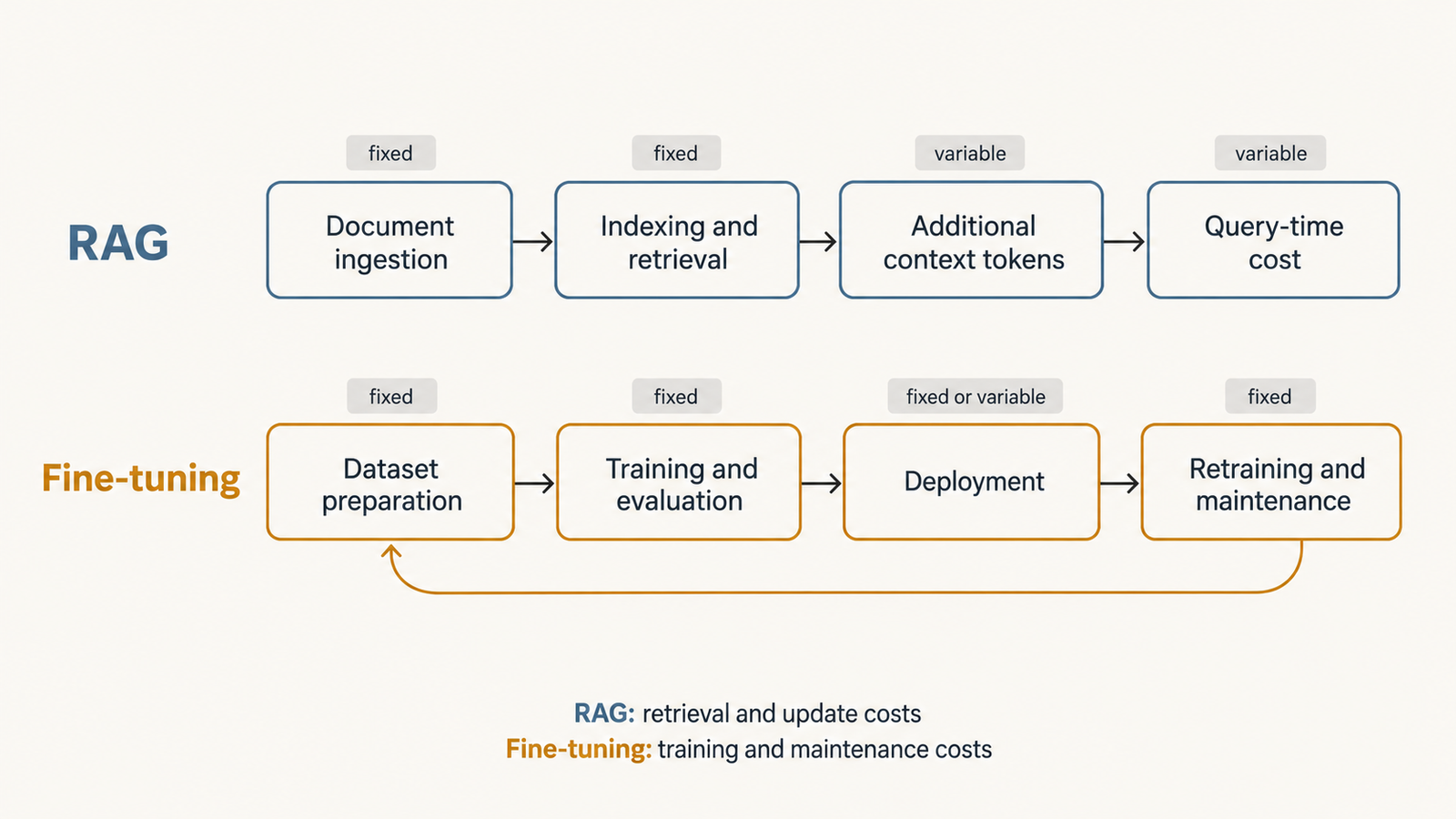
Checked against the burner22/numbat repository and its discussions, Hugging Face and PyTorch documentation, and Moonshot AI’s announcement on 2 November 2026. On 1 November, a …
Agentic AI Statistics

30 Agentic AI Statistics for 2026: Adoption, Spending and Risk

Last updated: 15 November 2026. This page is updated monthly; each figure keeps its original publication date. Agent traffic at one healthcare booking platform rose …