On September 22, 2026, Anthropic cut the price of its flagship Opus tier. Ninety minutes later, OpenAI halved the price of two GPT-6 models. Both announcements led with a percentage.
Percentages are the wrong unit. The invoice is denominated in tasks, and a task is a bundle of cached input, fresh input, output tokens, tool calls, retries and occasional failures that reach production. Change the mix and a 50% token-price cut can produce anything from a 50% saving to almost none.
This is a comparison of GPT-6 Sol vs Claude Opus 5.5 by workload shape rather than by rate card. The short version: the line that decides most agentic bills is the cached-input read, and on that line the two models are now priced identically.
Key takeaways
- Both models landed on September 22, 2026, about 90 minutes apart. GPT-6 Sol lists at $2/$10 per million input/output tokens; Claude Opus 5.5 at $4/$20.
- Cache reads are $0.20 per million on both. On cache-heavy agent workloads, the headline 2:1 token-price gap compresses sharply.
- The two “cheaper” claims use different baselines. OpenAI’s 50% is measured against GPT-5.6 promotional pricing; Anthropic’s 20% is against Opus 5, with the larger 40% figure resting on token efficiency at default settings.
- Output tokens, not input, dominate reasoning-heavy bills. A model that thinks longer can cost more per task at a lower per-token price.
- Neither company published a symmetric head-to-head. OpenAI benchmarked Sol against Claude Opus 5 and, where 5.1 numbers were missing, Fable 5, using competitor scores from published reports.
- Token prices fell while memory prices rose: TrendForce recorded conventional DRAM contract prices up 93–98% quarter over quarter in Q1 2026 before moderating to 13–18% in Q3.
- The only reliable comparison is your own traffic. Cost per completed task, measured on 50 real inputs, beats any published rate card.
Quick Navigation
- GPT-6 Sol vs Claude Opus 5.5: The Numbers Everyone Is Comparing
- Where the GPT-6 Sol vs Claude Opus 5.5 Savings Actually Come From
- The Cache Line That Changes the GPT-6 Sol vs Claude Opus 5.5 Math
- Five Workload Shapes Where GPT-6 Sol vs Claude Opus 5.5 Diverges
- Why Infrastructure Costs Tell a Different Story
- Memory Is Becoming Part of the Token Price
- The GPT-6 Sol vs Claude Opus 5.5 Benchmark Comparison Has a Catch
- Run the 50-Request GPT-6 Sol vs Claude Opus 5.5 Test
- A Practical Cost Model for GPT-6 Sol vs Claude Opus 5.5 Buyers
- Failure Shape: Where Cheap Tokens Get Expensive
- What the Price War Actually Changed
- Frequently Asked Questions
GPT-6 Sol vs Claude Opus 5.5: The Numbers Everyone Is Comparing
Here is what each company published, kept in separate categories, because list price, promotional price, batch price and cached price are not interchangeable.
| Line item (per 1M tokens) | GPT-6 Sol | Claude Opus 5.5 |
|---|---|---|
| Input | $2.00 | $4.00 |
| Output | $10.00 | $20.00 |
| Cached input read | $0.20 | $0.20 |
| Cache write (5-min) | No separate charge published | $5.00 |
| Cache write (1-hour) | Not applicable | $8.00 |
| Batch | 50% off | $2.00 / $10.00 |
| Fast / premium mode | Not offered at this tier | $8.00 / $40.00 |
| Predecessor | GPT-5.6 Sol at $4 / $20 | Claude Opus 5 at $5 / $25 |
OpenAI’s announcement states the reduction plainly: Sol moves from $4/$20 to $2/$10 and Luna from $0.20/$1.20 to $0.10/$0.50, a 50% cut against GPT-5.6 promotional pricing, attributed to caching and inference improvements the company says it is passing on. Cached input-token reads carry a 90% discount, which puts Sol’s cached reads at $0.20.
Anthropic’s Opus 5.5 lists at $4 input and $20 output, down from Opus 5’s $5 and $25, with cache reads falling from $0.50 to $0.20 and five-minute cache writes from $6.25 to $5. Anthropic told reporters the model runs about 40% cheaper than Opus 5 at default settings, combining the 20% token-price cut with fewer tokens consumed per task.
Two caveats before anyone builds a spreadsheet on these numbers. OpenAI’s baseline is a promotional rate, not a long-standing list price, so “50% cheaper” compares against a discount that was already in force. An OpenAI spokesperson told VentureBeat the new rates are permanent rather than promotional; that is a company statement, not something a buyer can verify from outside. And Anthropic’s 40% is a blended claim about workloads, not a line on the rate card — the rate card says 20%.
Verify both against the live pricing pages before you commit a budget. Rate cards move, and the ones above were published on launch day.
Where the GPT-6 Sol vs Claude Opus 5.5 Savings Actually Come From
A price cut can arrive through three different doors, and they behave differently on your invoice.
- Door one: the per-token rate. This is the headline. It applies uniformly to every token of the relevant class, so a 50% cut here does produce a 50% saving — but only on the portion of the bill made of tokens priced at that rate.
- Door two: the discount structure. Cached reads, batch processing and long-context surcharges change which rate applies to which tokens. This door moves more money than the first one on most production workloads, and almost nobody reads it.
- Door three: token efficiency. If a model completes the same task using fewer output tokens, the bill falls without any rate changing. Anthropic leaned on this explicitly, saying Opus 5.5 generates output faster and uses fewer tokens per task. Efficiency claims are the hardest to verify from outside, because they depend on your prompts and your effort settings.
The distinction matters because doors two and three are workload-dependent, while door one is not. Two teams on identical rate cards can see completely different savings.
The Cache Line That Changes the GPT-6 Sol vs Claude Opus 5.5 Math
Cached input reads cost $0.20 per million tokens on both models. That single equality does more to determine competitive cost than the 2:1 gap on list input price, because of what modern agents actually send.
An agent turn is mostly repetition. The system instructions, the tool schemas, the retrieved documents, the repository context and the conversation so far all get resent on every turn. Only the newest user message and the model’s reply are genuinely new. On a long-running agent, cached tokens routinely outnumber fresh ones by an order of magnitude.
Work through what that does to a single turn. Take 100,000 tokens of reused prefix, 5,000 tokens of new input and 1,500 tokens of output. This is a worked example, not a measurement.
| Component | GPT-6 Sol | Claude Opus 5.5 |
|---|---|---|
| 100,000 cached input | $0.0200 | $0.0200 |
| 5,000 fresh input | $0.0100 | $0.0200 |
| 1,500 output | $0.0150 | $0.0300 |
| Turn total | $0.0450 | $0.0700 |
Sol is about 36% cheaper on that turn, not 50%. Now run the same prefix uncached: 105,000 input tokens cost $0.21 on Sol against $0.42 on Opus 5.5, and the full 2:1 ratio returns — along with a bill roughly five times larger on both.
The caching mechanism differs in ways that matter operationally. OpenAI applies caching automatically to eligible reused prefixes within a rolling window and publishes no separate write charge, while giving developers explicit breakpoints, a caching dashboard and a diagnostics tool, plus the ability to change reasoning effort or toggle tools mid-conversation without invalidating the cached prefix. Anthropic charges for cache writes — $5 per million for the five-minute window, $8 for the one-hour window — which means the break-even depends on how many reads each write earns.
That write charge is not a disadvantage so much as a different shape. A prefix written once and read forty times amortizes cheaply. A prefix written once and read twice does not. If your agent rebuilds its context frequently, model the writes explicitly.
The efficiency gains are real on the provider side too. OpenAI says GitHub reported that its caching improvements cut the share of prompt tokens needing fresh processing by more than half, measured across billions of requests. That is a claim about one large customer’s traffic, reported by OpenAI, and it says nothing about what your cache-hit rate will be.
Five Workload Shapes Where GPT-6 Sol vs Claude Opus 5.5 Diverges
Every calculation below is a labelled hypothetical built from published rates. None of it is measured production data, and your token counts will differ.
1. Long-context agentic work
A research or operations agent holding 150,000 tokens of context, running 12 turns, producing 2,000 output tokens per turn. Most input is cached after the first turn.
The cached portion is priced identically on both, so the comparison collapses to output and fresh input. Sol’s advantage is real but roughly a third, not a half. Anthropic’s cache-write charge applies on each rebuild of the prefix; if the agent’s context shifts every few turns, add $0.75 per rebuild on a 150,000-token prefix at the five-minute rate.
2. High-volume classification and extraction
Short inputs, short outputs, millions of requests, little or no reuse. Say 800 input tokens and 120 output tokens per call, 5 million calls a month.
| GPT-6 Sol | Claude Opus 5.5 | |
|---|---|---|
| Input, 4B tokens | $8,000 | $16,000 |
| Output, 600M tokens | $6,000 | $12,000 |
| Monthly total | $14,000 | $28,000 |
This is the shape where the headline ratio holds exactly, because nothing is cached and nothing is reasoned about at length. It is also the shape where neither of these models is the right answer — GPT-6 Luna at $0.10/$0.50 would run the same volume for roughly $700, and the real question is whether its accuracy clears your threshold.
3. Coding agents with heavy cache reuse
A coding agent maintaining 200,000 tokens of repository context across 30 turns, 1,500 output tokens per turn, cache hit rate above 90%.
Here the bill is dominated by cached reads at $0.20 on both sides, plus output. Sol wins on output price; Opus 5.5 wins if Anthropic’s token-efficiency claim holds on your tasks, because fewer thinking tokens beats a lower price per thinking token. This is precisely the case where the rate card cannot answer the question and a measured test can.
4. One-shot generation
20,000 tokens in, 2,000 out, no reuse. Sol costs $0.06, Opus 5.5 costs $0.12. Clean 2:1, and the absolute numbers are small enough that the choice should probably rest on output quality rather than price.
5. Repeated multi-step agent loops
The shape where estimates go wrong. Ten tool calls per task, each one a model round trip, each carrying the accumulated trace. Costs compound with the square of the loop length as the transcript grows, and a single retried loop can double a task’s cost.
This is also where reasoning-token volume bites. Independent testing reported by Artificial Analysis put Opus 5.5 at the top of its Intelligence Index as of September 22, while consuming roughly 119,000 output tokens per task against about 73,000 for Opus 5 and 27,000 for GPT-6 Astra. Read carefully: that is a cross-model figure from one evaluation suite, not a measurement of your agent. But it illustrates the mechanism — a model that reasons longer can produce a larger bill at a lower per-token rate, and the effort setting you choose moves this number more than the rate card does.
The pattern
| Workload shape | Where cost concentrates | Does the 2:1 price gap hold? |
|---|---|---|
| Long-context agentic | Cached reads, output | No, compresses sharply |
| High-volume extraction | Fresh input, output | Yes |
| Coding agent, high reuse | Cached reads, output | No, and token efficiency may reverse it |
| One-shot generation | Fresh input, output | Yes |
| Multi-step loops | Output, retries | Unpredictable without measurement |
Why Infrastructure Costs Tell a Different Story
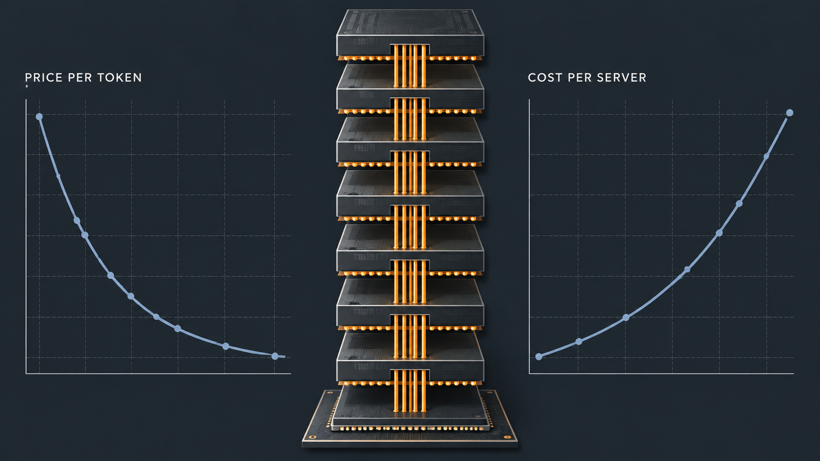
Token prices halved in September. The inputs to serving those tokens did not.
Memory is the clearest case. TrendForce’s contract-price surveys recorded conventional DRAM rising roughly 93–98% quarter over quarter in Q1 2026, lifting industry revenue 81% to about $97 billion, followed by a further 58–63% in Q2. By Q3 the increase moderated to 13–18% quarter over quarter, with server DRAM undersupplied and suppliers prioritising AI and server allocations. Moderating growth on top of two near-doublings is still a much higher price than a year earlier.
Keep the categories distinct, because they are not substitutes and they do not move together:
| Category | What it is | Where it sits |
|---|---|---|
| Conventional DRAM | Standard DDR5 memory | Server main memory, consumer devices |
| Server DRAM / RDIMM | Registered modules for servers | Host memory beside accelerators |
| HBM | Stacked high-bandwidth memory | On the accelerator package |
| GPU memory | The HBM attached to a specific accelerator | Holds weights and KV cache |
HBM is allocated separately from conventional DRAM and priced separately, but they compete for the same wafers. TrendForce noted suppliers reallocating capacity toward HBM and server products, which is part of why commodity memory repriced so violently.
So how do providers cut prices into that? Three mechanisms, none of which requires hardware to get cheaper: better utilisation of accelerators already deployed, architectural and serving efficiency improvements, and margin. OpenAI attributes its reduction to caching and inference improvements. That is a credible mechanism and also a commercial decision — Ramp’s lead economist described the two labs as fighting a price war that is driving down both AI prices and their own ability to profit from it.
The useful inference for a buyer: today’s rate card reflects a competitive position, not a cost floor. Build your model so a rate change in either direction does not invalidate it.
Memory Is Becoming Part of the Token Price
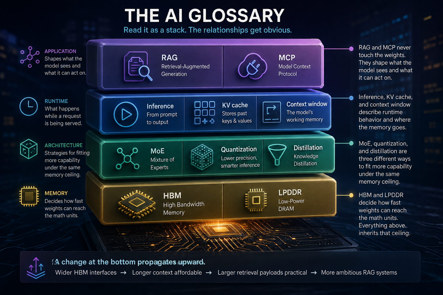
Generating tokens is a memory-bound problem, and that is why caching is priced the way it is.
During decoding, the accelerator reads the model weights and the KV cache — the stored attention state for every token in the context — for each token it produces. Arithmetic units sit idle waiting for data. Throughput is governed by how fast bytes move out of HBM, not by peak FLOPS.
That has three consequences for anyone reading a price sheet.
- Context length is a memory cost, not just a token cost. KV cache size grows linearly with context. A 200,000-token prefix occupies real HBM for the duration of the request, and that capacity cannot serve anyone else. This is why long-context tiers carry surcharges: reported pricing for Sol applies a 2x input and 1.5x output multiplier above 272,000 input tokens, which is worth confirming against the API docs if your workload runs long.
- A cache read is cheap because the expensive part already happened. The prefill computation that built the attention state was paid for on the write. The read reuses stored state, which is closer to a memory-and-storage operation than a compute one. That is the physical reason both vendors landed near $0.20 rather than near their input prices.
- Batching is where provider economics live. Serving many requests concurrently amortises the weight reads across more output tokens. Latency-sensitive, low-batch workloads are the expensive ones to serve, which is why batch APIs carry 50% discounts and why fast modes cost double.
None of this changes what you are billed per token. It explains why the structure of the price sheet looks the way it does, and why the cheap line is cheap.
The GPT-6 Sol vs Claude Opus 5.5 Benchmark Comparison Has a Catch
Neither company published a head-to-head against the other’s new model. They could not have: the two launched ninety minutes apart.
OpenAI’s comparisons are mostly cost per task rather than cost per token, which is the right unit, and they name Anthropic repeatedly. On AutomationBench 1.0.6, GPT-6 Sol at xhigh effort scored 33.2% at $0.27 per task, against Claude Opus 5 at max effort on 26.9% at 11.1 times Sol’s cost per task. On DeepSWE v1.1, Sol at max effort scored 68.8%, within 1.1 points of Claude Fable 5’s 69.9% at xhigh, at roughly 80% lower cost per task. On OSWorld 2.0 offline, Sol at xhigh scored 60.5% against Opus 5 at medium on 60.3%, again at about 80% lower cost.
Read OpenAI’s own footnotes before reading the charts. The company states that competitor scores were taken from publicly available reports rather than run in-house, and that Claude Fable 5 scores stood in where Fable 5.1 numbers were unavailable. It also notes that its Fable 5.1 AutomationBench datapoint understates that model’s real cost, because it omits the Opus 5 fallbacks that fired on roughly 40% of tasks.
So the baseline is Claude Opus 5, the model Opus 5.5 replaced. None of those comparisons touch Opus 5.5.
Anthropic’s side has the mirror problem. Its launch table put Opus 5.5 at 66.4% on Terminal-Bench 4.0 against 52.3% for Opus 5 and 57.9% for GPT-6 Astra — a different benchmark, a different generation of competitor, and a different effort configuration.
Three things make these numbers non-comparable:
- Different baselines. OpenAI measured against Opus 5 and Fable 5; Anthropic measured against Opus 5, Fable 5.1 and GPT-6 Astra.
- Different effort settings. “xhigh”, “max” and “medium” are not equivalent, and effort drives both score and cost. A comparison at mismatched effort levels is a comparison of two configurations, not two models.
- Different evaluation suites and versions. AutomationBench 1.0.6, DeepSWE v1.1, OSWorld v2026.08.08 and Terminal-Bench 4.0 measure different things.
Company-reported results are evidence about what a vendor could demonstrate under conditions it chose. Independent head-to-head evaluation is a different category, and at the time of writing the independent picture is thin — Artificial Analysis had run both, placing Opus 5.5 at the top of its Intelligence Index on September 22, at a notably high output-token cost per task.
We are not declaring a winner on this evidence, because the evidence does not support one. What it does support is narrower and more useful: cost per task varies by an order of magnitude across effort settings on the same model, which means your effort configuration is a bigger cost lever than your model choice.
Run the 50-Request GPT-6 Sol vs Claude Opus 5.5 Test
Take 50 representative inputs from your actual traffic — not curated examples, not the ones you already know work — and run them through both models at the effort settings you would ship. Then measure eight things:
- Cost per request, broken into cached input, fresh input and output
- p95 latency, not mean latency
- Output tokens consumed per request
- Cache-hit rate and cache-read volume
- Retry rate
- Failure rate
- The split between obvious failures and silent ones
- Task completion rate against your own definition of complete
Call this a practical screening experiment. Fifty inputs will not give you statistical confidence, and anyone who tells you otherwise is selling something. What it will give you is the distribution shape: whether one model’s costs cluster tightly while the other’s have a long tail, whether failures announce themselves or slip through, and whether the effort setting you assumed is the right one.
Fifty is enough to catch the things leaderboards structurally cannot show you. Benchmarks report aggregate accuracy on someone else’s task distribution. They do not report what happens when your particular malformed PDF arrives, or how many output tokens your prompt style provokes, or whether the model quietly returns a plausible wrong answer instead of an error.
Run it again after any prompt change. Cache-hit rates are fragile, and a small edit to a system prompt can invalidate a prefix and quietly multiply your input bill.
A Practical Cost Model for GPT-6 Sol vs Claude Opus 5.5 Buyers
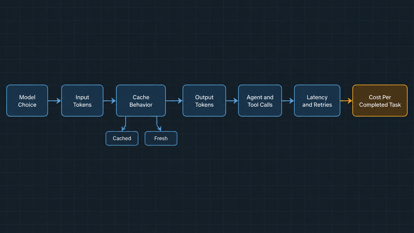
Cost per million tokens is not cost per completed business task. Here is the arithmetic that gets you from one to the other.
Cost per request = (cached input tokens × cache-read rate) + (fresh input tokens × input rate) + (cache-write tokens × write rate) + (output tokens × output rate)
Cost per completed task = (cost per request × requests per task × (1 + retry rate)) ÷ task completion rate
The denominator is what most spreadsheets omit. A model that completes 90% of tasks costs you 1.11 times its nominal per-task price, before anyone accounts for the human who handles the other 10%.
Measure these inputs before you model anything:
| Input | Why it matters |
|---|---|
| Input tokens per request | Sets the base, and splits into cached and fresh |
| Cached input tokens per request | The line priced identically across both models |
| Cache-hit rate | Moves the bill more than the rate card does |
| Output tokens per request | Dominates reasoning-heavy workloads |
| Requests per task | Agent loops multiply everything upstream |
| Retry rate | Adds cost without adding completions |
| Task completion rate | Converts cost per request into cost per outcome |
| p95 latency | Determines whether batch pricing is available to you |
| Tool-call count | Each call is another round trip carrying the transcript |
Two structural options are worth testing before you negotiate anything. Batch processing is half price on both platforms and is available to any workload that tolerates delay — reporting, enrichment, overnight classification. And tiering is usually cheaper than choosing: route the easy majority to a small model and reserve the expensive tier for what needs it. GPT-6 Luna at $0.10/$0.50 exists precisely for that split.
Failure Shape: Where Cheap Tokens Get Expensive
Two models can post the same accuracy and impose completely different operational costs, because accuracy is a count and failure is a distribution.
Five failure types, in rough order of how much they cost you:
| Type | What it looks like | Who absorbs it |
|---|---|---|
| Explicit refusal or error | The call fails visibly | Your retry logic |
| Partial completion | Half the job, clearly incomplete | A human, quickly |
| Tool-use failure | The agent loops or stalls on a call | Your token budget |
| Plausible but wrong output | Confident, well-formatted, incorrect | A reviewer, if you have one |
| Wrong output reaching a downstream system | Nobody notices until later | The business |
The first three are cheap because they are loud. They cost tokens and latency, both of which show up in the metrics you already watch.
The last two are the expensive ones, and their cost has nothing to do with token prices. An incorrect classification that routes a support ticket wrongly costs a few minutes. An incorrect figure in a financial summary that someone acts on costs considerably more. An incorrect medical code creates a billing and compliance problem that surfaces weeks later. An incorrect customer email cannot be recalled. An incorrect code change that passes review reaches production.
Run the arithmetic on a realistic case. A workload processing 100,000 tasks a month at $0.05 per task costs $5,000. A silent error rate of 0.5% produces 500 wrong outputs. If each one costs $50 to detect and remediate — a conservative figure in regulated work — that is $25,000, five times the inference bill. Halving the token price saves $2,500. Halving the silent error rate saves $12,500.
That is the whole argument for measuring failure shape before optimising price.
We are not claiming either model has a particular failure tendency; the published evidence does not support that kind of claim, and failure profiles are heavily prompt-dependent. OpenAI does report that Sol makes about half as many factual mistakes as GPT-5.6 Sol on an internal evaluation, while noting that the evaluation is drawn from conversations users flagged as erroneous and is not representative of typical use. That is a claim about one model against its own predecessor, on a deliberately error-prone set.
What matters for your decision is which failure types your architecture can absorb. If a human reviews every output, plausible-but-wrong is survivable. If the output writes to a ledger, it is not, and you should be paying for whatever reduces it.
What the Price War Actually Changed
Three things changed on September 22, and two things did not.
- Changed: the floor for frontier-adjacent capability. Work that cost $4 per million input tokens in August costs $2 now on OpenAI’s side, and the Opus tier came down 20%. That is real, and it makes workloads viable that were not.
- Changed: cache reads became a commodity. At $0.20 on both platforms, the cached-input line is no longer a differentiator. Vendors now compete on hit rates, cache controls and write economics rather than on the read price itself.
- Changed: the unit of comparison. OpenAI’s own announcement leads with cost per task rather than cost per token. When the seller changes units, the buyer should too.
- Unchanged: the cost of being wrong. Nothing in either rate card touches remediation.
- Unchanged: the direction of infrastructure costs. Memory repriced upward through 2026 while token prices fell. Providers are absorbing that gap through efficiency and margin, which means today’s prices reflect a competitive moment rather than a durable cost structure.
The practical conclusion for a buyer comparing GPT-6 Sol vs Claude Opus 5.5 is unglamorous. Instrument your workload, measure cached versus fresh input, measure output tokens at the effort setting you will actually ship, and compute cost per completed task rather than cost per million tokens. The rate card is the least informative document in this decision.
Frequently Asked Questions
Which is cheaper, GPT-6 Sol or Claude Opus 5.5?
On list price, Sol at $2/$10 per million tokens is half of Opus 5.5 at $4/$20. On a cache-heavy agent workload the gap narrows substantially, because cached reads cost $0.20 on both. On any workload, the answer depends on output-token volume at your effort setting.
Do cache reads really cost the same on both?
Yes, at $0.20 per million tokens as of the September 22, 2026 launches. The structures differ: OpenAI applies a 90% cached-read discount automatically within a reuse window and publishes no separate write charge, while Anthropic charges $5 per million for a five-minute cache write and $8 for a one-hour write.
Why doesn’t a 50% price cut halve my bill?
Because only the tokens priced at the cut rate get the discount. Cached reads, batch-processed tokens and long-context surcharges follow different lines, and retries, tool calls and failed tasks add cost that no rate card mentions.
What does cache-hit rate do to cost?
More than almost anything else. Moving 100,000 tokens of prefix from fresh to cached takes that line from $0.20 to $0.02 on Sol, and from $0.40 to $0.02 on Opus 5.5. Small prompt edits can invalidate a prefix and silently reverse the saving.
How should I price long-context workloads?
Count the KV cache, not just the tokens. Long prefixes occupy accelerator memory for the life of the request, which is why surcharges exist above certain thresholds — reported at 2x input and 1.5x output above 272,000 input tokens for Sol. Confirm current thresholds in the API documentation.
Keep reading
Here are the latest posts from the blog.

GPT-6 Sol vs Claude Opus 5.5: What the 50% Cut Misses

Employee-Level Evaluator Access: The Security Problem Nobody Priced

Pacing the Frontier: What It Actually Does to AI Chip Demand