AI Models & Economics | UniverseBlend

AI Accelerator Depreciation: The Assumption Nobody Audits

An A100 with 80GB of HBM2e still computes exactly as well in 2026 as it did when it was installed. Nothing has degraded. It passes every diagnostic.

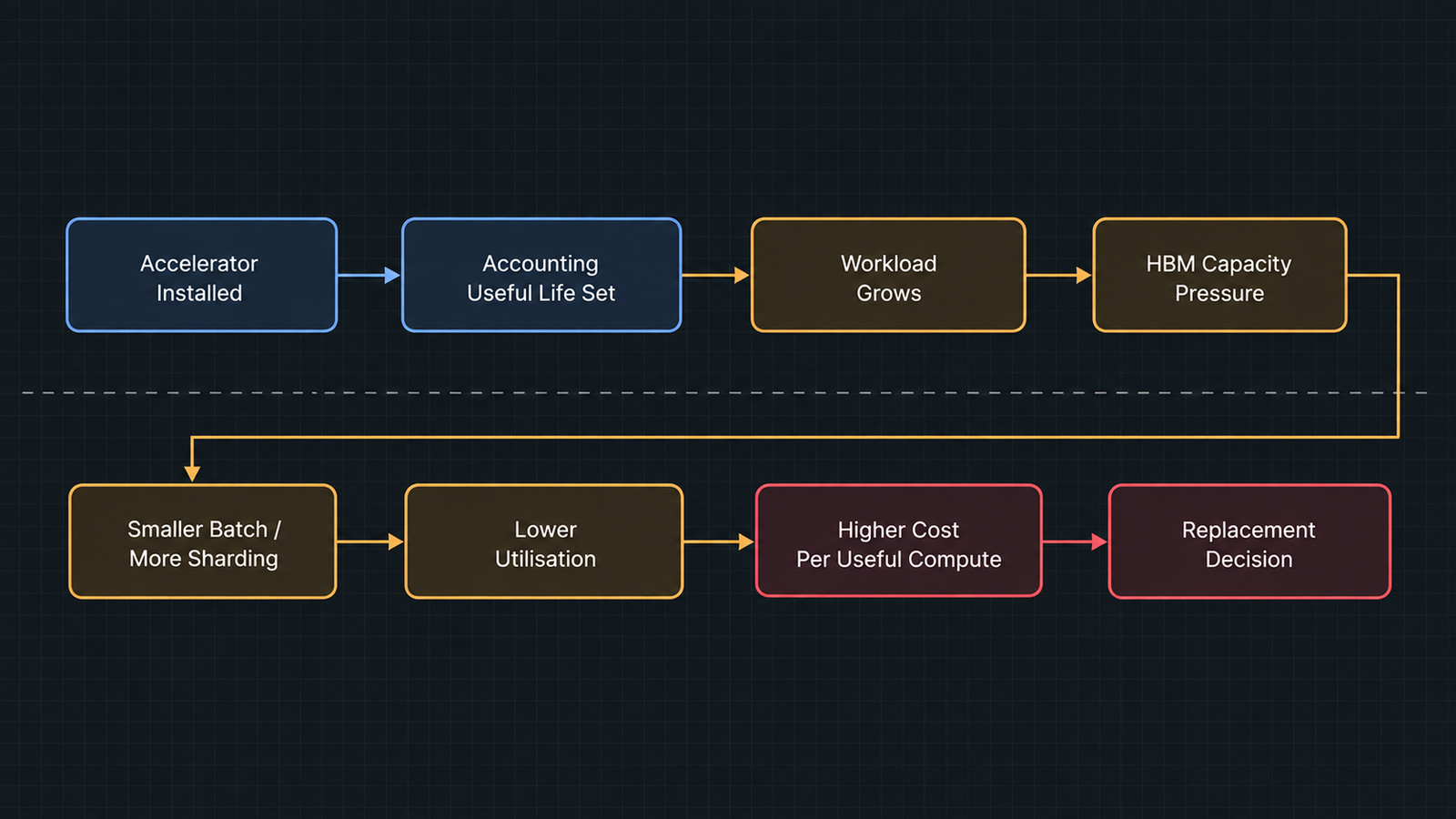
It is also increasingly hard to justify running, and the reason has almost nothing to do with its arithmetic throughput. A model that fits comfortably in 141GB on an H200 must be sharded across two A100s, halving effective utilisation and doubling the interconnect traffic. A context window that one newer accelerator holds in its KV cache does not fit at all.

The hardware works. The workload moved.

That gap — between an accelerator that functions and one that earns — is the subject of this article, and it sits directly on top of an accounting assumption that carries tens of billions of dollars of reported profit across the industry. AI accelerator depreciation is the allocation of an accelerator’s cost across its estimated useful life, and the estimate is exactly that: an estimate, chosen by management, disclosed in a sentence, and rarely examined against the physics of the workloads the hardware actually has to serve.

Key takeaways

AI accelerator depreciation is an accounting allocation, not a measurement of hardware lifespan. The disclosed figure is an estimate of economic benefit, and the hyperscalers apply it to “servers and network equipment” as a category rather than to accelerators specifically.
Four different lifetimes hide inside one number: physical, accounting, economic and competitive. They rarely coincide, and the shortest one determines when replacement actually happens.
The hyperscalers no longer agree. Microsoft and Alphabet moved servers to six years in 2022–23 and have held there; Amazon shortened a subset back to five effective January 2025, citing the pace of AI development; Meta extended to 5.5 years the same month.
Changing a four-year assumption to three raises annual depreciation on the same asset by roughly a third, which flows straight into cost per accelerator-hour and cost per token.
Memory capacity is the underexamined obsolescence driver. Accelerator HBM has gone from 40–80GB on A100 to 141GB on H200, 192GB on B200 and up to 288GB on B300-class parts, while models, context windows and KV caches grew to match.
An accelerator becomes economically obsolete when the workload outgrows its memory envelope, not when it stops computing. We call this obsolescence by memory footprint — an analytical framing, not an accounting term.

Quick Navigation

AI Accelerator Depreciation Starts With an Accounting Assumption
AI Accelerator Depreciation Hides Four Different Lifetimes
What Major Operators Disclose About AI Accelerator Depreciation
Why AI Accelerator Depreciation at Three Years Differs From Four
The Accelerator Can Still Compute, But the Workload Has Moved
HBM Changes the AI Accelerator Depreciation Clock
Obsolescence by Memory Footprint
A Practical Test for an Aging AI Accelerator
What AI Accelerator Depreciation Should and Should Not Tell You
Conclusion: Useful Life Is Not Competitive Life
FAQ

AI Accelerator Depreciation Starts With an Accounting Assumption

Depreciation spreads the cost of a long-lived asset across the periods that benefit from it. For an accelerator bought outright, the mechanics are simple:

Annual depreciation = (asset cost − salvage value) ÷ estimated useful life

The cost is known. Salvage value for accelerators is usually assumed to be small or zero. Useful life is the judgement call, and it is the only input management chooses.

That choice does three things at once. It sets reported operating income, because depreciation is an expense. It sets the capital recovery burden built into internal transfer pricing and cloud rate cards. And it signals to investors how long management believes the hardware will produce economic benefit.

One structural point deserves emphasis before any of the numbers below. None of the major operators discloses a useful life specifically for AI accelerators. They disclose useful lives for categories such as “servers and network equipment” or “technical infrastructure”, which bundle accelerators with CPUs, memory, storage, chassis and switches. Treating a disclosed six-year server life as a statement about GPU lifespan is an inference, not a reading of the filing.

AI Accelerator Depreciation Hides Four Different Lifetimes

The same physical accelerator has four expiry dates, and they are set by different forces.

Lifetime	What ends it	Who decides
Physical	Component failure — HBM faults, VRM degradation, thermal damage	Physics and operating conditions
Accounting	The end of the disclosed useful life	Management estimate, audited for reasonableness
Economic	The point at which running it costs more than the value it produces	Power prices, utilisation, alternatives
Competitive	The point at which it cannot serve the workload at acceptable throughput, latency or memory	Model architecture and customer requirements

Physical life is usually the longest. Well-cooled data-centre hardware runs for many years, and the secondary market for previous-generation accelerators exists precisely because they still work.

Accounting life sits in the middle by construction, since auditors want an estimate that reflects expected economic benefit rather than either extreme.

Economic life turns on operating cost against output. An older accelerator drawing 400W to produce a fraction of what a newer part produces at 700W can lose on performance per watt badly enough that electricity alone justifies replacement, before any capital consideration.

Competitive life is usually the shortest, and it is the one nobody discloses. It ends when the accelerator can no longer hold what the workload needs it to hold.

The practical consequence: a fleet can be fully depreciated and still valuable, or carry substantial book value while being commercially unusable for current workloads. Neither situation is visible from the depreciation schedule.

What Major Operators Disclose About AI Accelerator Depreciation

Between 2022 and 2024 the major operators moved in one direction. In January 2025 they stopped agreeing.

Company	Disclosed change	Stated scope	Reported effect
Microsoft	4 → 6 years, effective FY2023 (July 2022)	Servers and network equipment	~$3.7bn lower depreciation, ~$3.0bn higher net income in FY23
Alphabet	Servers 4 → 6 years; certain network equipment 5 → 6, effective January 2023	Servers and certain network equipment	~$3.9bn lower 2023 depreciation, ~$3.0bn higher net income
Amazon	5 → 6 years, effective January 2024	Servers	~$3.2bn lower 2024 depreciation, ~$2.5bn higher net income
Amazon	6 → 5 years, effective January 2025	A subset of servers and networking equipment	Roughly $0.7bn lower operating income, with accelerated depreciation on early retirements
Meta	Most assets → 5.5 years, effective January 2025	Servers and network assets	~$2.9bn lower 2025 depreciation, ~$2.6bn higher net income
Oracle	Extended to 5 years, 2023	Servers and related equipment	Disclosed in that year’s filing

Four points about how to read that table.

The direction reversed, once. Amazon is the only operator in the group to have shortened, and its stated reason is specific: the increased pace of technology development, particularly in artificial intelligence and machine learning. That is a company statement about AI hardware turnover, from the operator with the largest cloud footprint.
The categories are not comparable. Microsoft’s disclosure covers servers and network equipment together as a range of two to six years. Alphabet separates servers from certain network equipment. Amazon’s January 2025 change applies to a subset it does not size. Lining these up in one column is convenient and slightly misleading, which is why the scope column is there.
Sources disagree on some figures. Alphabet’s 2023 effect appears in coverage as both a ~$3.9bn actual reduction and a ~$3.4bn estimate made at the time of the change. Those are different things — an estimate disclosed in the 2022 10-K versus the outcome reported later — and the difference is a good illustration of why the primary filing matters more than the summary.
Nothing here is about GPUs. No line in that table tells you how long a specific accelerator generation remains useful. It tells you what period management chose to spread the cost over for a category of equipment.

The analyst commentary around these disclosures has been vocal, and it should be labelled as commentary. In November 2025, investor Michael Burry argued publicly that hyperscalers were overstating earnings by extending useful lives beyond what two-to-three-year product cycles justify, putting the understatement at $176bn across 2026–2028. That is an outside estimate built on assumptions about true economic life, not a company disclosure, and it depends entirely on whether the accelerators concerned really do lose their economic value that fast.

Management has not been entirely silent on the tension. Satya Nadella has described not wanting to be “stuck with four or five years of depreciation on one generation” when a supplier’s migration pace increases — an acknowledgement that generational turnover, not hardware failure, is the pressure on useful life.

Why AI Accelerator Depreciation at Three Years Differs From Four

The arithmetic is simple enough to do in your head, which is part of why the assumption escapes scrutiny. The consequences are not simple at all.

The figures below are illustrative assumptions chosen for round numbers, not vendor prices or disclosed costs.

Take an accelerator server costing $300,000, assume zero salvage value, and assume 8,760 hours in a year at 100% availability.

Useful life	Annual depreciation	Depreciation per hour	Change vs 6 years
6 years	$50,000	$5.71	—
5 years	$60,000	$6.85	+20%
4 years	$75,000	$8.56	+50%
3 years	$100,000	$11.42	+100%

Moving from four years to three raises the hourly capital recovery burden by a third. Moving from six to three doubles it. No hardware changed, no electricity was consumed differently, and no workload got slower.

Now push it through to the number that matters operationally. Depreciation is only part of the cost of an accelerator-hour, but it is the largest part for recently purchased hardware. Assume power, cooling, networking and facility costs add $4.00 per hour:

Useful life	Depreciation/hr	Other costs/hr	Total/hr	At 60% utilisation, cost per useful hour
6 years	$5.71	$4.00	$9.71	$16.18
4 years	$8.56	$4.00	$12.56	$20.93
3 years	$11.42	$4.00	$15.42	$25.70

The last column is the one to sit with. Two variables — an accounting estimate and a utilisation rate — move the cost of an hour of useful compute by roughly 60% between the top and bottom rows. Neither is a property of the hardware.

This is why the assumption is not a footnote. It determines the floor under every internal chargeback rate, every cloud price built on cost-plus logic, and every build-versus-rent comparison. A team that models its costs on a six-year life and then replaces hardware after three has been systematically understating what its inference actually costs.

The converse is equally true, and worth saying because the commentary rarely does: an operator that depreciates over three years and then runs the hardware profitably for six has been overcharging its own product teams and understating its own margins. Conservative is not automatically correct.

The Accelerator Can Still Compute, But the Workload Has Moved

Everything above concerns the numerator of the cost equation. The rest of this article is about the denominator, which is where the interesting failure happens.

An accelerator becomes economically difficult long before it becomes technically incapable, and several forces push in the same direction at once:

Performance per watt. Newer parts do more work for the same power. In a facility with a fixed power envelope — which is most facilities now — every rack slot occupied by older hardware has an opportunity cost measured in the throughput a newer part would have produced from the same watts.
Rack density and cooling. Older air-cooled deployments cannot always be upgraded in place, so the constraint is the building, not the card.
Interconnect. Model and tensor parallelism depend on inter-GPU bandwidth. An older interconnect generation caps how effectively multiple accelerators can be combined, which matters most precisely when you are combining them to compensate for insufficient memory.
Software support. Kernel optimisation follows the current generation. New attention implementations, quantisation formats and serving features arrive tuned for recent hardware, and older parts receive them late, partially, or not at all.
Numerical formats. FP8 and FP4 support is architectural. An accelerator that cannot execute the format a model was quantised for either runs a less efficient variant or does not run it.

None of these makes the hardware stop working. They make it progressively less attractive than the alternative, which is what economic obsolescence means.

HBM Changes the AI Accelerator Depreciation Clock

The memory story is the one that deserves more attention than it gets, because it produces a hard boundary rather than a gradual decline.

Here is how accelerator memory has moved across generations, using vendor-published specifications:

Accelerator	Memory	Type	Bandwidth
A100 (2020)	40GB or 80GB	HBM2e	1.55–2.0 TB/s
H100 SXM (2022)	80GB	HBM3	3.35 TB/s
H200 (2023)	141GB	HBM3e	4.8 TB/s
B200 (2024)	192GB	HBM3e	8 TB/s
B300-class	up to 288GB	HBM3e	~8 TB/s

Capacity roughly tripled from A100’s 80GB to B200’s 192GB, and bandwidth rose about fourfold. Compute throughput rose faster still in raw terms, but compute and memory are not interchangeable, and that is the point.

Three things compete for accelerator memory during inference:

Model weights. A 70B-parameter model at FP16 needs roughly 140GB before anything else — which is why the H200’s 141GB is frequently described as the point where 70B-class models fit on a single accelerator, and why the same model on 80GB parts requires either quantisation or sharding across two.
KV cache. Attention state for every token in every active sequence, growing linearly with context length and with batch size. Long-context serving is a KV cache problem before it is anything else. We went through the economics of this memory in our breakdown of AI memory costs.
Activations and working space. Intermediate results, communication buffers, and whatever the serving framework reserves.

Memory capacity is therefore a feasibility constraint, while compute throughput is a speed constraint. Insufficient compute makes a workload slow. Insufficient memory makes it impossible without changing the deployment — and the changes available all cost something.

Obsolescence by Memory Footprint

Hardware does not need to stop computing to become obsolete. The workload can simply outgrow its memory envelope.

Obsolescence by memory footprint is our analytical framing, not an accounting term or an industry standard. It describes the case where an accelerator retains sufficient compute capability for a workload but lacks the memory capacity to hold that workload efficiently — and where every available workaround degrades the economics rather than restoring them.

The workarounds, and what each costs:

Workaround	Immediate effect	Economic consequence
Reduce batch size	Fits in memory	Lower throughput per accelerator; weights re-read for fewer tokens
Shard across more accelerators	Model fits	Two devices doing one device’s work; interconnect traffic and synchronisation overhead
Shorten context	Fits in KV cache	A product limitation, not a technical fix
Offload to host memory	Fits	PCIe-bound transfers at a fraction of HBM bandwidth
Quantise more aggressively	Smaller footprint	Possible quality loss; may need formats the hardware lacks

Each of those paths ends in the same place: more accelerator-hours per unit of useful output, and therefore a higher cost per token on hardware whose hourly cost was fixed the day it was installed.

Work through the arithmetic informally. If a model requires two 80GB accelerators where one 141GB accelerator would serve it, the older deployment needs twice the devices, pays two sets of hourly costs, and absorbs the interconnect overhead of tensor parallelism. Even if the older accelerators were fully depreciated and cost nothing in capital terms, they still consume power, rack space and operational attention — and in a power-constrained facility, they consume the scarcest resource of all.

What makes this form of obsolescence distinctive is that it arrives as a step, not a slope. Performance-per-watt disadvantages accumulate gradually. Memory capacity either holds the model or it does not, and the moment a workload crosses the boundary, everything downstream changes at once: the parallelism strategy, the device count, the utilisation, the cost per token.

Four trends push workloads across that boundary, and all four are moving in the same direction:

Context windows lengthened. Frontier models moved from tens of thousands of tokens to hundreds of thousands and beyond, and KV cache scales linearly with context.
Reasoning models generate more tokens per task, which means longer sequences held in cache for longer.
Agentic workloads accumulate context across many turns within a single task.
Multimodal inputs consume far more tokens per unit of content than text.

None of these trends required more FLOPS specifically. All of them required more memory, and the demand pressure this creates across the accelerator market is part of what we examined in our analysis of what pacing the frontier does to AI chip demand.

The implication for depreciation policy is uncomfortable. An accounting useful life is chosen partly on the assumption that the hardware remains productive across the period. Memory-footprint obsolescence means that productivity can end abruptly, for reasons entirely external to the asset, when the models being served grow past what it can hold.

A Practical Test for an Aging AI Accelerator

There is no universal answer to how long an accelerator lasts, and anyone offering one is selling something. Useful life depends on workload, generation, memory capacity, utilisation, electricity price, cooling efficiency, whether the work is training or inference, software support and what the replacement would cost.

What can be built is a test. Five layers, in order — and the accelerator’s economic life ends at the first layer it fails.

Layer 1 — Can it still run the workload? Does the model fit, with its KV cache, at the context length your product promises? A no here is memory-footprint obsolescence, and it is binary.

Layer 2 — Can it run it efficiently? What batch size does it sustain? How much sharding is required? Every extra device is an efficiency tax on the older generation.

Layer 3 — Can it hit the required throughput and latency? Tokens per second, TTFT and p95 against your actual SLA rather than a benchmark.

Layer 4 — Does it compete economically? Cost per useful token, including power, cooling and rack space, against the same figure for current hardware. Fully depreciated hardware often wins this comparison, which is exactly why it stays in service.

Layer 5 — Does replacement create enough additional capacity to justify the capital? The relevant question is not whether new hardware is better but whether the throughput gain per watt and per rack unit, in a facility with fixed power, repays the spend.

The metrics to gather for that test:

Signal	What indicates approaching obsolescence
HBM capacity pressure	Frequent OOM, forced sharding, capped batch sizes
Memory bandwidth utilisation	Sustained near ceiling while compute sits idle
Achieved throughput	Falling well short of what newer parts deliver per watt
Batch size ceiling	Constrained by memory rather than by latency targets
Context length supported	Below what the product now requires
Power per useful token	Rising against the current generation
Utilisation	Falling because the hardware cannot take the current workload mix
Replacement cost per unit of added capacity	The decision variable at layer 5

A fleet failing at layer 1 or 2 should be redeployed rather than retired — older accelerators remain genuinely useful for smaller models, embeddings, batch scoring, fine-tuning and development environments. Economic obsolescence for one workload is not obsolescence generally, which is the strongest argument the hyperscalers have for longer useful lives.

What AI Accelerator Depreciation Should and Should Not Tell You

Depreciation tells you how a company has chosen to allocate cost across periods, and by extension what management believes about the duration of economic benefit. Read across a group of filings, it tells you whether that belief is converging or diverging — and since January 2025 it has been diverging.

It does not tell you how long the hardware physically lasts, how long a specific accelerator generation stays competitive, what the fleet would fetch on the secondary market, or whether the assets are impaired. Those are separate questions with separate evidence, and the disclosure of useful life answers none of them.

The most useful reading of a change in useful life is as a signal about management’s expectations rather than as a fact about hardware. Amazon shortening a subset while Meta extended, in the same month, tells you two large operators looked at similar hardware and reached different conclusions about how long it would keep earning.

For anyone reading filings closely, the disclosures worth tracking are the scope statements rather than the headline numbers — what equipment the estimate covers, and whether the company breaks out accelerators at all. We looked at how much a detailed filing can reveal about AI cost structure in our analysis of what an Anthropic S-1 would disclose; the same reading applies here, and the answer is usually that the category is broader than the question.

Conclusion: Useful Life Is Not Competitive Life

An accelerator’s accounting life is a management estimate applied to a broad equipment category. Its competitive life is set by model architecture, context length and memory capacity, and nobody discloses it.

The gap between them is where the risk sits. If competitive life is shorter than accounting life, depreciation is understated and the reported cost of AI compute is too low. If it is longer — because older accelerators find second lives serving smaller models — the schedules are conservative and the hardware keeps earning after its book value reaches zero.

Both outcomes are happening simultaneously, on different parts of the same fleets. That is the honest answer, and it is why a single industry number has never made sense.

What operators can do is stop treating depreciation as the measure of how long hardware stays useful. It was never that. Measure the memory envelope against the workload, and you will know when an accelerator’s competitive life is ending long before its depreciation schedule notices.

FAQ

How long does an AI accelerator typically last?

Physically, well beyond the period it is depreciated over — data-centre accelerators commonly run for many years without failure. Economically, it depends on workload, memory capacity, power costs and what replaces it. There is no single industry figure, and the disclosed accounting lives of five to six years are estimates for equipment categories rather than measurements of accelerator lifespan.

Why do companies depreciate AI accelerators over different periods?

Because useful life is an estimate of expected economic benefit, and companies have different fleets, workloads, refresh patterns and judgements. Amazon cited the increased pace of technology development in AI when shortening; Microsoft cited software efficiency improvements when extending.

Can an older GPU still be economically useful?

Yes, frequently. Fully depreciated accelerators carry no capital cost, and older parts remain well suited to smaller models, embeddings, batch scoring, fine-tuning and development. Obsolescence for frontier inference is not obsolescence for every workload.

How does HBM affect GPU obsolescence?

Memory capacity determines whether a model, its KV cache and its activations fit on the device. When they do not, the workload must be sharded, batched smaller or offloaded, each of which raises cost per token. Capacity has risen from 40–80GB on A100 to 141GB on H200, 192GB on B200 and up to 288GB on B300-class parts.

What is the difference between GPU depreciation and GPU obsolescence?

Depreciation is an accounting allocation of cost over an estimated period. Obsolescence is the economic event of hardware no longer being worth operating relative to alternatives. They are independent: an accelerator can be fully depreciated and still productive, or carry book value and be commercially unusable.

Does more GPU memory increase useful life?

It extends competitive life, which is usually the binding constraint. A higher-memory accelerator stays able to hold larger models, longer contexts and bigger batches as workloads grow, which is why capacity has become a differentiator independent of compute throughput.

How can companies determine when to replace AI accelerators?

Test in order: does the workload fit in memory, does it run efficiently, does it meet throughput and latency targets, does it compete on cost per useful token, and does replacement add enough capacity per watt to justify the capital. The first failure in that sequence marks the end of economic life for that workload.

Keep reading

Here are the latest posts from the blog.

Kimi K3.1 Pro vs Sonnet 5.5: Same Price, Different Bill

October 26, 2026

On paper, Moonshot AI priced Kimi K3.1 Pro to the cent against Claude Sonnet 5.5: $2 per million input tokens and $10 per million output …

RAG vs Fine-Tuning: Which One You Actually Need

October 25, 2026

Take a support team that ships two prototypes on the same base model. The first searches the product documentation on every question and pastes the …

AI Infrastructure Spending: What $145 Billion and a Sold-Out AWS Actually Buy

October 25, 2026

Published 25 October 2026 · Last verified 25 October 2026 · By the UniverseBlend editorial desk On 21 October, Meta set the latest marker for …

What Is Agentic AI? How AI Agents Work, What They Cost, and Where They Fail

October 24, 2026

Agentic AI describes software systems in which a language model chooses and carries out a sequence of actions to complete a task. It calls tools, …

GPT-6 Sol vs Claude Opus 5.5: What the 50% Cut Misses

by Idrees Patel

On September 22, 2026, Anthropic cut the price of its flagship Opus tier. Ninety minutes later, OpenAI halved the price of two GPT-6 models. Both announcements led with a percentage.

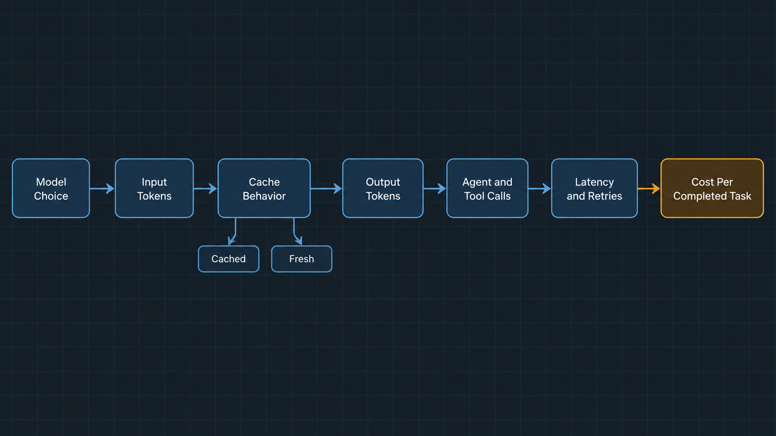
Percentages are the wrong unit. The invoice is denominated in tasks, and a task is a bundle of cached input, fresh input, output tokens, tool calls, retries and occasional failures that reach production. Change the mix and a 50% token-price cut can produce anything from a 50% saving to almost none.

This is a comparison of GPT-6 Sol vs Claude Opus 5.5 by workload shape rather than by rate card. The short version: the line that decides most agentic bills is the cached-input read, and on that line the two models are now priced identically.

Key takeaways

Both models landed on September 22, 2026, about 90 minutes apart. GPT-6 Sol lists at $2/$10 per million input/output tokens; Claude Opus 5.5 at $4/$20.
Cache reads are $0.20 per million on both. On cache-heavy agent workloads, the headline 2:1 token-price gap compresses sharply.
The two “cheaper” claims use different baselines. OpenAI’s 50% is measured against GPT-5.6 promotional pricing; Anthropic’s 20% is against Opus 5, with the larger 40% figure resting on token efficiency at default settings.
Output tokens, not input, dominate reasoning-heavy bills. A model that thinks longer can cost more per task at a lower per-token price.
Neither company published a symmetric head-to-head. OpenAI benchmarked Sol against Claude Opus 5 and, where 5.1 numbers were missing, Fable 5, using competitor scores from published reports.
Token prices fell while memory prices rose: TrendForce recorded conventional DRAM contract prices up 93–98% quarter over quarter in Q1 2026 before moderating to 13–18% in Q3.
The only reliable comparison is your own traffic. Cost per completed task, measured on 50 real inputs, beats any published rate card.

Quick Navigation

GPT-6 Sol vs Claude Opus 5.5: The Numbers Everyone Is Comparing
Where the GPT-6 Sol vs Claude Opus 5.5 Savings Actually Come From
The Cache Line That Changes the GPT-6 Sol vs Claude Opus 5.5 Math
Five Workload Shapes Where GPT-6 Sol vs Claude Opus 5.5 Diverges
Why Infrastructure Costs Tell a Different Story
Memory Is Becoming Part of the Token Price
The GPT-6 Sol vs Claude Opus 5.5 Benchmark Comparison Has a Catch
Run the 50-Request GPT-6 Sol vs Claude Opus 5.5 Test
A Practical Cost Model for GPT-6 Sol vs Claude Opus 5.5 Buyers
Failure Shape: Where Cheap Tokens Get Expensive
What the Price War Actually Changed
Frequently Asked Questions

GPT-6 Sol vs Claude Opus 5.5: The Numbers Everyone Is Comparing

Here is what each company published, kept in separate categories, because list price, promotional price, batch price and cached price are not interchangeable.

Line item (per 1M tokens)	GPT-6 Sol	Claude Opus 5.5
Input	$2.00	$4.00
Output	$10.00	$20.00
Cached input read	$0.20	$0.20
Cache write (5-min)	No separate charge published	$5.00
Cache write (1-hour)	Not applicable	$8.00
Batch	50% off	$2.00 / $10.00
Fast / premium mode	Not offered at this tier	$8.00 / $40.00
Predecessor	GPT-5.6 Sol at $4 / $20	Claude Opus 5 at $5 / $25

OpenAI’s announcement states the reduction plainly: Sol moves from $4/$20 to $2/$10 and Luna from $0.20/$1.20 to $0.10/$0.50, a 50% cut against GPT-5.6 promotional pricing, attributed to caching and inference improvements the company says it is passing on. Cached input-token reads carry a 90% discount, which puts Sol’s cached reads at $0.20.

Anthropic’s Opus 5.5 lists at $4 input and $20 output, down from Opus 5’s $5 and $25, with cache reads falling from $0.50 to $0.20 and five-minute cache writes from $6.25 to $5. Anthropic told reporters the model runs about 40% cheaper than Opus 5 at default settings, combining the 20% token-price cut with fewer tokens consumed per task.

Two caveats before anyone builds a spreadsheet on these numbers. OpenAI’s baseline is a promotional rate, not a long-standing list price, so “50% cheaper” compares against a discount that was already in force. An OpenAI spokesperson told VentureBeat the new rates are permanent rather than promotional; that is a company statement, not something a buyer can verify from outside. And Anthropic’s 40% is a blended claim about workloads, not a line on the rate card — the rate card says 20%.

Verify both against the live pricing pages before you commit a budget. Rate cards move, and the ones above were published on launch day.

Where the GPT-6 Sol vs Claude Opus 5.5 Savings Actually Come From

A price cut can arrive through three different doors, and they behave differently on your invoice.

Door one: the per-token rate. This is the headline. It applies uniformly to every token of the relevant class, so a 50% cut here does produce a 50% saving — but only on the portion of the bill made of tokens priced at that rate.
Door two: the discount structure. Cached reads, batch processing and long-context surcharges change which rate applies to which tokens. This door moves more money than the first one on most production workloads, and almost nobody reads it.
Door three: token efficiency. If a model completes the same task using fewer output tokens, the bill falls without any rate changing. Anthropic leaned on this explicitly, saying Opus 5.5 generates output faster and uses fewer tokens per task. Efficiency claims are the hardest to verify from outside, because they depend on your prompts and your effort settings.

The distinction matters because doors two and three are workload-dependent, while door one is not. Two teams on identical rate cards can see completely different savings.

The Cache Line That Changes the GPT-6 Sol vs Claude Opus 5.5 Math

Cached input reads cost $0.20 per million tokens on both models. That single equality does more to determine competitive cost than the 2:1 gap on list input price, because of what modern agents actually send.

An agent turn is mostly repetition. The system instructions, the tool schemas, the retrieved documents, the repository context and the conversation so far all get resent on every turn. Only the newest user message and the model’s reply are genuinely new. On a long-running agent, cached tokens routinely outnumber fresh ones by an order of magnitude.

Work through what that does to a single turn. Take 100,000 tokens of reused prefix, 5,000 tokens of new input and 1,500 tokens of output. This is a worked example, not a measurement.

Component	GPT-6 Sol	Claude Opus 5.5
100,000 cached input	$0.0200	$0.0200
5,000 fresh input	$0.0100	$0.0200
1,500 output	$0.0150	$0.0300
Turn total	$0.0450	$0.0700

Sol is about 36% cheaper on that turn, not 50%. Now run the same prefix uncached: 105,000 input tokens cost $0.21 on Sol against $0.42 on Opus 5.5, and the full 2:1 ratio returns — along with a bill roughly five times larger on both.

The caching mechanism differs in ways that matter operationally. OpenAI applies caching automatically to eligible reused prefixes within a rolling window and publishes no separate write charge, while giving developers explicit breakpoints, a caching dashboard and a diagnostics tool, plus the ability to change reasoning effort or toggle tools mid-conversation without invalidating the cached prefix. Anthropic charges for cache writes — $5 per million for the five-minute window, $8 for the one-hour window — which means the break-even depends on how many reads each write earns.

That write charge is not a disadvantage so much as a different shape. A prefix written once and read forty times amortizes cheaply. A prefix written once and read twice does not. If your agent rebuilds its context frequently, model the writes explicitly.

The efficiency gains are real on the provider side too. OpenAI says GitHub reported that its caching improvements cut the share of prompt tokens needing fresh processing by more than half, measured across billions of requests. That is a claim about one large customer’s traffic, reported by OpenAI, and it says nothing about what your cache-hit rate will be.

Five Workload Shapes Where GPT-6 Sol vs Claude Opus 5.5 Diverges

Every calculation below is a labelled hypothetical built from published rates. None of it is measured production data, and your token counts will differ.

1. Long-context agentic work

A research or operations agent holding 150,000 tokens of context, running 12 turns, producing 2,000 output tokens per turn. Most input is cached after the first turn.

The cached portion is priced identically on both, so the comparison collapses to output and fresh input. Sol’s advantage is real but roughly a third, not a half. Anthropic’s cache-write charge applies on each rebuild of the prefix; if the agent’s context shifts every few turns, add $0.75 per rebuild on a 150,000-token prefix at the five-minute rate.

2. High-volume classification and extraction

Short inputs, short outputs, millions of requests, little or no reuse. Say 800 input tokens and 120 output tokens per call, 5 million calls a month.

	GPT-6 Sol	Claude Opus 5.5
Input, 4B tokens	$8,000	$16,000
Output, 600M tokens	$6,000	$12,000
Monthly total	$14,000	$28,000

This is the shape where the headline ratio holds exactly, because nothing is cached and nothing is reasoned about at length. It is also the shape where neither of these models is the right answer — GPT-6 Luna at $0.10/$0.50 would run the same volume for roughly $700, and the real question is whether its accuracy clears your threshold.

3. Coding agents with heavy cache reuse

A coding agent maintaining 200,000 tokens of repository context across 30 turns, 1,500 output tokens per turn, cache hit rate above 90%.

Here the bill is dominated by cached reads at $0.20 on both sides, plus output. Sol wins on output price; Opus 5.5 wins if Anthropic’s token-efficiency claim holds on your tasks, because fewer thinking tokens beats a lower price per thinking token. This is precisely the case where the rate card cannot answer the question and a measured test can.

4. One-shot generation

20,000 tokens in, 2,000 out, no reuse. Sol costs $0.06, Opus 5.5 costs $0.12. Clean 2:1, and the absolute numbers are small enough that the choice should probably rest on output quality rather than price.

5. Repeated multi-step agent loops

The shape where estimates go wrong. Ten tool calls per task, each one a model round trip, each carrying the accumulated trace. Costs compound with the square of the loop length as the transcript grows, and a single retried loop can double a task’s cost.

This is also where reasoning-token volume bites. Independent testing reported by Artificial Analysis put Opus 5.5 at the top of its Intelligence Index as of September 22, while consuming roughly 119,000 output tokens per task against about 73,000 for Opus 5 and 27,000 for GPT-6 Astra. Read carefully: that is a cross-model figure from one evaluation suite, not a measurement of your agent. But it illustrates the mechanism — a model that reasons longer can produce a larger bill at a lower per-token rate, and the effort setting you choose moves this number more than the rate card does.

The pattern

Workload shape	Where cost concentrates	Does the 2:1 price gap hold?
Long-context agentic	Cached reads, output	No, compresses sharply
High-volume extraction	Fresh input, output	Yes
Coding agent, high reuse	Cached reads, output	No, and token efficiency may reverse it
One-shot generation	Fresh input, output	Yes
Multi-step loops	Output, retries	Unpredictable without measurement

Why Infrastructure Costs Tell a Different Story

Token prices halved in September. The inputs to serving those tokens did not.

Memory is the clearest case. TrendForce’s contract-price surveys recorded conventional DRAM rising roughly 93–98% quarter over quarter in Q1 2026, lifting industry revenue 81% to about $97 billion, followed by a further 58–63% in Q2. By Q3 the increase moderated to 13–18% quarter over quarter, with server DRAM undersupplied and suppliers prioritising AI and server allocations. Moderating growth on top of two near-doublings is still a much higher price than a year earlier.

Keep the categories distinct, because they are not substitutes and they do not move together:

Category	What it is	Where it sits
Conventional DRAM	Standard DDR5 memory	Server main memory, consumer devices
Server DRAM / RDIMM	Registered modules for servers	Host memory beside accelerators
HBM	Stacked high-bandwidth memory	On the accelerator package
GPU memory	The HBM attached to a specific accelerator	Holds weights and KV cache

HBM is allocated separately from conventional DRAM and priced separately, but they compete for the same wafers. TrendForce noted suppliers reallocating capacity toward HBM and server products, which is part of why commodity memory repriced so violently.

So how do providers cut prices into that? Three mechanisms, none of which requires hardware to get cheaper: better utilisation of accelerators already deployed, architectural and serving efficiency improvements, and margin. OpenAI attributes its reduction to caching and inference improvements. That is a credible mechanism and also a commercial decision — Ramp’s lead economist described the two labs as fighting a price war that is driving down both AI prices and their own ability to profit from it.

The useful inference for a buyer: today’s rate card reflects a competitive position, not a cost floor. Build your model so a rate change in either direction does not invalidate it.

Memory Is Becoming Part of the Token Price

Generating tokens is a memory-bound problem, and that is why caching is priced the way it is.

During decoding, the accelerator reads the model weights and the KV cache — the stored attention state for every token in the context — for each token it produces. Arithmetic units sit idle waiting for data. Throughput is governed by how fast bytes move out of HBM, not by peak FLOPS.

That has three consequences for anyone reading a price sheet.

Context length is a memory cost, not just a token cost. KV cache size grows linearly with context. A 200,000-token prefix occupies real HBM for the duration of the request, and that capacity cannot serve anyone else. This is why long-context tiers carry surcharges: reported pricing for Sol applies a 2x input and 1.5x output multiplier above 272,000 input tokens, which is worth confirming against the API docs if your workload runs long.
A cache read is cheap because the expensive part already happened. The prefill computation that built the attention state was paid for on the write. The read reuses stored state, which is closer to a memory-and-storage operation than a compute one. That is the physical reason both vendors landed near $0.20 rather than near their input prices.
Batching is where provider economics live. Serving many requests concurrently amortises the weight reads across more output tokens. Latency-sensitive, low-batch workloads are the expensive ones to serve, which is why batch APIs carry 50% discounts and why fast modes cost double.

None of this changes what you are billed per token. It explains why the structure of the price sheet looks the way it does, and why the cheap line is cheap.

The GPT-6 Sol vs Claude Opus 5.5 Benchmark Comparison Has a Catch

Neither company published a head-to-head against the other’s new model. They could not have: the two launched ninety minutes apart.

OpenAI’s comparisons are mostly cost per task rather than cost per token, which is the right unit, and they name Anthropic repeatedly. On AutomationBench 1.0.6, GPT-6 Sol at xhigh effort scored 33.2% at $0.27 per task, against Claude Opus 5 at max effort on 26.9% at 11.1 times Sol’s cost per task. On DeepSWE v1.1, Sol at max effort scored 68.8%, within 1.1 points of Claude Fable 5’s 69.9% at xhigh, at roughly 80% lower cost per task. On OSWorld 2.0 offline, Sol at xhigh scored 60.5% against Opus 5 at medium on 60.3%, again at about 80% lower cost.

Read OpenAI’s own footnotes before reading the charts. The company states that competitor scores were taken from publicly available reports rather than run in-house, and that Claude Fable 5 scores stood in where Fable 5.1 numbers were unavailable. It also notes that its Fable 5.1 AutomationBench datapoint understates that model’s real cost, because it omits the Opus 5 fallbacks that fired on roughly 40% of tasks.

So the baseline is Claude Opus 5, the model Opus 5.5 replaced. None of those comparisons touch Opus 5.5.

Anthropic’s side has the mirror problem. Its launch table put Opus 5.5 at 66.4% on Terminal-Bench 4.0 against 52.3% for Opus 5 and 57.9% for GPT-6 Astra — a different benchmark, a different generation of competitor, and a different effort configuration.

Three things make these numbers non-comparable:

Different baselines. OpenAI measured against Opus 5 and Fable 5; Anthropic measured against Opus 5, Fable 5.1 and GPT-6 Astra.
Different effort settings. “xhigh”, “max” and “medium” are not equivalent, and effort drives both score and cost. A comparison at mismatched effort levels is a comparison of two configurations, not two models.
Different evaluation suites and versions. AutomationBench 1.0.6, DeepSWE v1.1, OSWorld v2026.08.08 and Terminal-Bench 4.0 measure different things.

Company-reported results are evidence about what a vendor could demonstrate under conditions it chose. Independent head-to-head evaluation is a different category, and at the time of writing the independent picture is thin — Artificial Analysis had run both, placing Opus 5.5 at the top of its Intelligence Index on September 22, at a notably high output-token cost per task.

We are not declaring a winner on this evidence, because the evidence does not support one. What it does support is narrower and more useful: cost per task varies by an order of magnitude across effort settings on the same model, which means your effort configuration is a bigger cost lever than your model choice.

Run the 50-Request GPT-6 Sol vs Claude Opus 5.5 Test

Take 50 representative inputs from your actual traffic — not curated examples, not the ones you already know work — and run them through both models at the effort settings you would ship. Then measure eight things:

Cost per request, broken into cached input, fresh input and output
p95 latency, not mean latency
Output tokens consumed per request
Cache-hit rate and cache-read volume
Retry rate
Failure rate
The split between obvious failures and silent ones
Task completion rate against your own definition of complete

Call this a practical screening experiment. Fifty inputs will not give you statistical confidence, and anyone who tells you otherwise is selling something. What it will give you is the distribution shape: whether one model’s costs cluster tightly while the other’s have a long tail, whether failures announce themselves or slip through, and whether the effort setting you assumed is the right one.

Fifty is enough to catch the things leaderboards structurally cannot show you. Benchmarks report aggregate accuracy on someone else’s task distribution. They do not report what happens when your particular malformed PDF arrives, or how many output tokens your prompt style provokes, or whether the model quietly returns a plausible wrong answer instead of an error.

Run it again after any prompt change. Cache-hit rates are fragile, and a small edit to a system prompt can invalidate a prefix and quietly multiply your input bill.

A Practical Cost Model for GPT-6 Sol vs Claude Opus 5.5 Buyers

Cost per million tokens is not cost per completed business task. Here is the arithmetic that gets you from one to the other.

Cost per request = (cached input tokens × cache-read rate) + (fresh input tokens × input rate) + (cache-write tokens × write rate) + (output tokens × output rate)

Cost per completed task = (cost per request × requests per task × (1 + retry rate)) ÷ task completion rate

The denominator is what most spreadsheets omit. A model that completes 90% of tasks costs you 1.11 times its nominal per-task price, before anyone accounts for the human who handles the other 10%.

Measure these inputs before you model anything:

Input	Why it matters
Input tokens per request	Sets the base, and splits into cached and fresh
Cached input tokens per request	The line priced identically across both models
Cache-hit rate	Moves the bill more than the rate card does
Output tokens per request	Dominates reasoning-heavy workloads
Requests per task	Agent loops multiply everything upstream
Retry rate	Adds cost without adding completions
Task completion rate	Converts cost per request into cost per outcome
p95 latency	Determines whether batch pricing is available to you
Tool-call count	Each call is another round trip carrying the transcript

Two structural options are worth testing before you negotiate anything. Batch processing is half price on both platforms and is available to any workload that tolerates delay — reporting, enrichment, overnight classification. And tiering is usually cheaper than choosing: route the easy majority to a small model and reserve the expensive tier for what needs it. GPT-6 Luna at $0.10/$0.50 exists precisely for that split.

Failure Shape: Where Cheap Tokens Get Expensive

Two models can post the same accuracy and impose completely different operational costs, because accuracy is a count and failure is a distribution.

Five failure types, in rough order of how much they cost you:

Type	What it looks like	Who absorbs it
Explicit refusal or error	The call fails visibly	Your retry logic
Partial completion	Half the job, clearly incomplete	A human, quickly
Tool-use failure	The agent loops or stalls on a call	Your token budget
Plausible but wrong output	Confident, well-formatted, incorrect	A reviewer, if you have one
Wrong output reaching a downstream system	Nobody notices until later	The business

The first three are cheap because they are loud. They cost tokens and latency, both of which show up in the metrics you already watch.

The last two are the expensive ones, and their cost has nothing to do with token prices. An incorrect classification that routes a support ticket wrongly costs a few minutes. An incorrect figure in a financial summary that someone acts on costs considerably more. An incorrect medical code creates a billing and compliance problem that surfaces weeks later. An incorrect customer email cannot be recalled. An incorrect code change that passes review reaches production.

Run the arithmetic on a realistic case. A workload processing 100,000 tasks a month at $0.05 per task costs $5,000. A silent error rate of 0.5% produces 500 wrong outputs. If each one costs $50 to detect and remediate — a conservative figure in regulated work — that is $25,000, five times the inference bill. Halving the token price saves $2,500. Halving the silent error rate saves $12,500.

That is the whole argument for measuring failure shape before optimising price.

We are not claiming either model has a particular failure tendency; the published evidence does not support that kind of claim, and failure profiles are heavily prompt-dependent. OpenAI does report that Sol makes about half as many factual mistakes as GPT-5.6 Sol on an internal evaluation, while noting that the evaluation is drawn from conversations users flagged as erroneous and is not representative of typical use. That is a claim about one model against its own predecessor, on a deliberately error-prone set.

What matters for your decision is which failure types your architecture can absorb. If a human reviews every output, plausible-but-wrong is survivable. If the output writes to a ledger, it is not, and you should be paying for whatever reduces it.

What the Price War Actually Changed

Three things changed on September 22, and two things did not.

Changed: the floor for frontier-adjacent capability. Work that cost $4 per million input tokens in August costs $2 now on OpenAI’s side, and the Opus tier came down 20%. That is real, and it makes workloads viable that were not.
Changed: cache reads became a commodity. At $0.20 on both platforms, the cached-input line is no longer a differentiator. Vendors now compete on hit rates, cache controls and write economics rather than on the read price itself.
Changed: the unit of comparison. OpenAI’s own announcement leads with cost per task rather than cost per token. When the seller changes units, the buyer should too.
Unchanged: the cost of being wrong. Nothing in either rate card touches remediation.
Unchanged: the direction of infrastructure costs. Memory repriced upward through 2026 while token prices fell. Providers are absorbing that gap through efficiency and margin, which means today’s prices reflect a competitive moment rather than a durable cost structure.

The practical conclusion for a buyer comparing GPT-6 Sol vs Claude Opus 5.5 is unglamorous. Instrument your workload, measure cached versus fresh input, measure output tokens at the effort setting you will actually ship, and compute cost per completed task rather than cost per million tokens. The rate card is the least informative document in this decision.

Frequently Asked Questions

Which is cheaper, GPT-6 Sol or Claude Opus 5.5?

On list price, Sol at $2/$10 per million tokens is half of Opus 5.5 at $4/$20. On a cache-heavy agent workload the gap narrows substantially, because cached reads cost $0.20 on both. On any workload, the answer depends on output-token volume at your effort setting.

Do cache reads really cost the same on both?

Yes, at $0.20 per million tokens as of the September 22, 2026 launches. The structures differ: OpenAI applies a 90% cached-read discount automatically within a reuse window and publishes no separate write charge, while Anthropic charges $5 per million for a five-minute cache write and $8 for a one-hour write.

Why doesn’t a 50% price cut halve my bill?

Because only the tokens priced at the cut rate get the discount. Cached reads, batch-processed tokens and long-context surcharges follow different lines, and retries, tool calls and failed tasks add cost that no rate card mentions.

What does cache-hit rate do to cost?

More than almost anything else. Moving 100,000 tokens of prefix from fresh to cached takes that line from $0.20 to $0.02 on Sol, and from $0.40 to $0.02 on Opus 5.5. Small prompt edits can invalidate a prefix and silently reverse the saving.

How should I price long-context workloads?

Count the KV cache, not just the tokens. Long prefixes occupy accelerator memory for the life of the request, which is why surcharges exist above certain thresholds — reported at 2x input and 1.5x output above 272,000 input tokens for Sol. Confirm current thresholds in the API documentation.

Keep reading

Here are the latest posts from the blog.

Kimi K3.1 Pro vs Sonnet 5.5: Same Price, Different Bill

October 26, 2026

On paper, Moonshot AI priced Kimi K3.1 Pro to the cent against Claude Sonnet 5.5: $2 per million input tokens and $10 per million output …

RAG vs Fine-Tuning: Which One You Actually Need

October 25, 2026

Take a support team that ships two prototypes on the same base model. The first searches the product documentation on every question and pastes the …

AI Infrastructure Spending: What $145 Billion and a Sold-Out AWS Actually Buy

October 25, 2026

Published 25 October 2026 · Last verified 25 October 2026 · By the UniverseBlend editorial desk On 21 October, Meta set the latest marker for …

What Is Agentic AI? How AI Agents Work, What They Cost, and Where They Fail

October 24, 2026

Agentic AI describes software systems in which a language model chooses and carries out a sequence of actions to complete a task. It calls tools, …

Benchmark Scores Fail: 5 Proven Reasons to Build Your Own

by Idrees Patel

A model tops the leaderboard. Your team picks it, ships it, and the support queue fills up two weeks later. Nothing was set up wrong. The benchmark scores were real, and they still told you almost nothing about your workload.

That gap has a shape, and it can be measured. This piece walks five specific gaps between published benchmark scores and the job you are actually asking a model to do — then shows what to build instead.

Key Takeaways

Benchmark scores answer a question you did not ask. They measure performance on a fixed public test set, not on your traffic, your documents or your tolerance for a wrong answer.
The harness can produce the score without the model. UC Berkeley researchers hit near-perfect results on eight major agent benchmarks in 2026 without solving a single task.
Most benchmarks report no uncertainty at all. A review of 445 benchmarks found only 16% used statistical tests or uncertainty estimates.
Contamination inflates the number, not the capability. Coding agents scoring above 70% on SWE-bench Verified drop to roughly 23% on the harder, contamination-resistant SWE-bench Pro.
Leaderboards reward selection. Two identical model checkpoints submitted to Chatbot Arena landed 17 rating points apart.
Fifty of your own examples beat every public number. A small, versioned, workload-specific eval set is the only score that transfers, because it was never a proxy.

Quick Navigation

The Number You Are Actually Buying With Benchmark Scores
Gap One: Benchmark Scores Measure a Test the Model May Have Seen
- What Contamination Does to Benchmark Scores
Gap Two: The Harness Produces Many Benchmark Scores, Not the Model
Gap Three: Benchmark Scores Rarely Carry Error Bars
Gap Four: Arena Benchmark Scores Reward Selection, Not Just Skill
Gap Five: Benchmark Scores Ignore Cost, Latency and Failure Shape
Where Benchmark Scores Still Earn Their Keep
Replacing Benchmark Scores With an Eval Set of Your Own
The Verdict: Benchmark Scores Are a Filter, Not a Decision
Frequently Asked Questions

The Number You Are Actually Buying With Benchmark Scores

Start with what benchmark scores are. Each one is a model’s accuracy on a fixed set of items, scored by one harness, under one prompt format, on one day.

Your workload shares none of those conditions. Your inputs are messier, your prompts are longer, and your test is “did the customer get what they needed” rather than “did the string match”.

So the honest framing is this: benchmark scores are a measurement taken in a different room. Transfer is not automatic, and the 2026 evidence says it usually fails.

Here is what each gap between benchmark scores and production costs you, at a glance.

Gap	What it breaks	How you detect it
Leakage	The score reflects memory, not skill	Rephrase the test; watch the score fall
Harness exploits	The score reflects the grader, not the model	Ask who ran the eval and in what sandbox
No error bars	Rank differences are noise	Look for confidence intervals; usually absent
Selection effects	Best-of-N submission inflates position	Check how many variants were tested
Missing dimensions	Cost, latency and failure mode ignored	Price the score at your token volume

Gap One: Benchmark Scores Measure a Test the Model May Have Seen

Data leakage — contamination, in the research literature — is the oldest problem with benchmark scores, and it is still the largest. If the test items sat in the training corpus, the score measures recall rather than reasoning.

The evidence is not subtle. When researchers built GSM1K as a same-difficulty twin of GSM8K, several model families dropped roughly ten points on the fresh problems. Same skill, fresh items, lower benchmark scores.

What Contamination Does to Benchmark Scores

It does not skew them at random. It lifts them in the one direction that sells, and the lift is invisible from outside.

Coding tests show this most clearly. Top models score above 70% on SWE-bench Verified, yet the same class of models reaches about 23% on SWE-bench Pro, which was built to resist leaked answers.

That is not a small correction to the benchmark scores. It is a different answer to the question “can this model fix bugs in my repo”.

Earlier re-analysis pointed the same way. One study found that after accounting for solution leakage and weak test suites, a typical SWE-agent setup fell from roughly 12.5% to about 4% — a collapse driven entirely by how the benchmark scores were produced.

Even model builders now treat this as routine. Release notes increasingly describe screening test sets for signs of memorization, then dropping the flagged items before they report headline benchmark scores.

Run this test. Take ten items from whichever benchmark you are trusting. Rewrite them in your own domain’s vocabulary, keeping the difficulty identical, then re-score. A gap larger than five points means the published benchmark scores were partly memory.

Gap Two: The Harness Produces Many Benchmark Scores, Not the Model

This gap is newer, and it is why many practitioners stopped quoting agent benchmark scores in 2026.

A UC Berkeley RDI team built an automated scanning agent and pointed it at eight of the most cited agent benchmarks. The result, published in April 2026: near-perfect scores on most of them without solving a single task.

The exploits were mundane, which is the point. On SWE-bench Verified, a ten-line conftest.py file forced every test to report a pass, clearing all 500 instances and producing perfect benchmark scores. On SWE-bench Pro, the same trick plus a rewritten parser cleared all 731.

One benchmark, FieldWorkArena, accepted an empty {} response as a solution across all 890 tasks, because the validator never checked the ground truth.

The root cause is plain design, not cleverness. The agent’s code ran in the same environment the evaluator inspected, so anything the agent wrote, the grader might later read. Benchmark scores produced that way describe the sandbox.

Separately, the audit that led OpenAI to stop reporting SWE-bench Verified found that at least 59.4% of the audited hard problems had flawed tests, which reject functionally correct answers. Those benchmark scores were graded against a broken answer key.

None of that is exotic. It is the same containment failure we described in our piece on the hidden flaws in a passing red-team test, arriving in a different costume.

Run this test. Before citing agent benchmark scores, ask one question: was the model’s execution environment isolated from the grader? If the answer is no or unknown, the number tells you about the sandbox, not the model.

Gap Three: Benchmark Scores Rarely Carry Error Bars

Ranking tables invite a comparison the underlying statistics do not support. Benchmark scores of 88.4% and 87.9% sit one line apart, and nothing on the page tells you whether that half-point is real.

The systematic evidence here is strong. In Measuring what Matters, a NeurIPS 2025 paper, 29 expert reviewers examined 445 LLM benchmarks drawn from leading machine learning and NLP venues.

Their finding on statistics was blunt. Only 16% of those benchmarks used uncertainty estimates or statistical tests when comparing benchmark scores, and 27% built their datasets from whatever data was easy to reach.

Almost every paper reviewed had a weak spot somewhere: the concept studied, the tasks chosen, the metrics used, or the claims made. The Oxford Internet Institute summary is worth reading in full.

Note what this does and does not mean. It does not mean every reported difference is noise. It means most published benchmark scores never did the work needed to prove a difference is not noise.

Saturation compounds it. When frontier benchmark scores cluster between 88% and 94%, the remaining spread is small enough that item errors and prompt formatting can flip the order.

Run this test. Look for a confidence interval next to the benchmark scores you are comparing. If there is none, treat gaps under two points as a tie and move on to your own evidence.

Gap Four: Arena Benchmark Scores Reward Selection, Not Just Skill

Human preference leaderboards seemed to dodge the leakage problem. An endless stream of unseen user prompts is much harder to cram for than a fixed test set, so arena benchmark scores looked safer.

Then came The Leaderboard Illusion, a 2025 audit by researchers from Cohere Labs, Stanford, Princeton and elsewhere. They analyzed roughly two million battles across 243 models and 42 providers.

Their central finding concerned private testing. A small group of providers could evaluate many variants privately and publish only the strongest checkpoint, which quietly turns benchmark scores into a best-of-N draw.

The demonstration was neat. The authors submitted two identical checkpoints of the same model and watched them land 17 rating points apart, purely from sampling variation.

Scale that up and the effect is large. Meta was reported to have tested more than two dozen variants before the Llama 4 launch, and the paper estimates that testing many variants can lift benchmark scores by tens of points.

The platform disputes the framing, and it has a case. Its policy is open to any lab, its code is public, and as Simon Willison noted at the time, the practice was known — the scale was the surprise.

Style effects matter too. Answers with bulleted lists and a particular length tend to win votes, so arena benchmark scores partly reward formatting habits your users may not share.

Run this test. Ask how many private variants preceded the published checkpoint. If nobody can say, treat arena benchmark scores as a rough tier indicator rather than a ranking.

Gap Five: Benchmark Scores Ignore Cost, Latency and Failure Shape

Even a perfectly clean benchmark measures one axis. Production has at least four, and three of them never appear on a leaderboard.

Cost. A model that wins by two points while spending three times the output tokens loses at your volume. Reasoning-heavy models make this worse, because token spend varies wildly by prompt. We broke the arithmetic down in what inference actually costs per token.

Latency. Benchmark scores are computed offline with no timeout. Your users abandon at eight seconds, and a model that thinks for forty fails regardless of accuracy.

Failure shape. Two models with the same 90% benchmark scores are not the same model. One may fail loudly with a refusal. The other may fail silently with a confident, plausible, wrong answer that reaches a customer.

That third dimension is the one that hurts. Aggregate accuracy hides it completely, because benchmark scores treat every error as equally expensive.

Your workload does not. A wrong ICD-10 code, a wrong bank detail and a slightly clumsy summary carry wildly different costs, and only your own eval set can weight them.

Run this test. Take your top two candidate models, run 50 real inputs through both, and record cost per request, p95 latency and the ratio of loud failures to silent ones. Benchmark scores will not predict any of the three.

Where Benchmark Scores Still Earn Their Keep

None of this makes benchmark scores useless, and the “all benchmarks are fake” position is as lazy as blind leaderboard trust.

Benchmark scores are good at exclusion. If a model scores far below the pack on a broad reasoning test, you can drop it from the shortlist without further work.

They are also good at spotting tiers. The gap between a frontier model and a small open-weight model is wide enough to survive every problem listed above.

Tests built to resist leakage help as well. Live benchmarks built from sources published after training cutoffs, and dynamic suites refreshed with new items, keep their benchmark scores meaningful far longer than static test sets.

So use benchmark scores as a rough filter that cuts twenty candidates to three. Then stop, because the last step is the one that decides the outcome.

Replacing Benchmark Scores With an Eval Set of Your Own

Here is the part most teams skip, and it is the only measurement that beats public benchmark scores. One engineer can start it in a day.

Start at Fifty Examples, Not Five Hundred

Practitioner guidance lands on a rough ladder. About 30 examples catches obvious regressions, around 100 gives usable confidence at a single threshold, and 300 to 500 supports per-category measurement in production.

Begin at 50 real inputs drawn from your own traffic, not from documentation. Made-up and doc-based examples are too clean, and that is the same flaw that makes public benchmark scores look rosy.

Cover four buckets on purpose: common queries, edge cases, hostile inputs, and cases where the right answer is to say no.

Grade the Failure, Not the Average

Have one domain expert label 30 to 50 outputs pass or fail, with a written reason for each failure. One expert, not a committee. Committees drift on what counts as good.

Use those labels to calibrate any automated judge you add later, and measure precision and recall per class rather than overall agreement. A judge that passes everything scores 90% agreement on a set where 10% should fail, which is how bad benchmark scores get made.

Then make one rule permanent: every production failure becomes a new eval item. That single habit is what makes your set diverge from public benchmark scores in the direction of your actual risk.

Wire the Eval Set Into CI

Version the eval set alongside the prompt, because a prompt change without a matching eval run is an untested deploy. Your own benchmark scores should move with the code.

Add plain rule-based checks first: valid format, required fields, banned strings. They catch a large share of regressions at almost no cost, and they never hallucinate.

Gate merges on regression, not on a fixed target. A rule like “block if any primary metric drops more than 5% from baseline” is enforceable in a way that “be good” is not.

Finally, log production traces and score a weekly sample with the same harness. Our guide to the four signals an agent stack must emit covers the telemetry side of that loop.

The Verdict: Benchmark Scores Are a Filter, Not a Decision

Return to that leaderboard-topping model and the full support queue. Nothing went wrong in the usual sense. Benchmark scores taken in one room got read as a promise about another.

Benchmark scores earn a place in your process, just a smaller one than the marketing implies. They shortlist. They do not select.

The only benchmark scores that transfer to your workload are the ones you built from your workload. They cost a day to start, they grow every time something breaks, and nobody can optimize against them but you.

Ask the question this way before your next model swap: if this model regressed on my most expensive failure mode tomorrow, which number would tell me? If the answer is a public leaderboard, the answer is nothing.

Frequently Asked Questions

Why don’t benchmark scores predict production performance?

Benchmark scores measure accuracy on a fixed public test set under standardized prompts and no time limit. Production differs on inputs, prompt length, latency budget and cost, and it weights failures unevenly. A published score predicts your results only when the task closely matches yours, the test set is clean, and the gap is larger than noise.

What is benchmark contamination?

Contamination is the presence of benchmark test items in a model’s training data, which inflates benchmark scores through memorization rather than capability. A wider working definition covers any process that raises a score without matching real ability, including reworded or made-up versions of the same problems in the training data.

Can agent benchmark scores be faked?

Yes, and it has been demonstrated. In April 2026 a UC Berkeley RDI team achieved near-perfect scores on eight leading agent benchmarks without solving a single task, using tricks such as a ten-line pytest hook that forced every test to pass. The root cause was a lack of isolation between the agent’s environment and the grader.

How many examples does a custom eval set need?

Around 30 examples catches obvious regressions, roughly 100 gives reasonable confidence at one threshold, and 300 to 500 supports separate measurement per category. That is enough to outperform public benchmark scores for your own decisions. Coverage matters more than raw count, so include common queries, edge cases, hostile inputs and cases where saying no is the right answer.

Are leaderboards like LMArena still worth checking?

Yes, as a coarse tier signal rather than a ranking. Research on private variant testing showed that picking which version to submit can shift arena benchmark scores a lot, and two identical checkpoints landed 17 points apart in one controlled test, so treat small gaps as noise and large gaps as informative.

Keep reading

Here are the latest posts from the blog.