Agentic AI vs Generative AI: Cost, Risk and Control

agentic AI vs generative AI

Generative AI produces an output, such as text, code or an image, from a prompt and its context. Agentic AI is a system that uses a generative model to pursue a goal over several steps, calling tools and acting on the results until it finishes or is stopped.

So agentic AI vs generative AI isn’t a contest between two kinds of model. Most agents run on the same large language models (LLMs) as chat assistants. What changes is the system around the model: how many calls a task makes, what those calls may touch, what they cost together and what happens when one goes wrong. The sections below work through each difference with calculations you can rerun on your own numbers.

Key Takeaways
  • They aren’t rival model types. An agent is an application architecture that usually calls a generative model many times.
  • Repeated context dominates many agent bills. In our illustrative ten-call loop, 84% of input tokens were repeats.
  • Token price isn’t task cost. In a hypothetical comparison, a model at one-third of the token price cost about 38% more per completed task.
  • Caching helps only when it hits. Cache writes cost more than ordinary input, so a loop that keeps missing the cache pays extra.
  • Actions outlive answers. Validation, idempotency and approval gates belong outside the model.
  • Instructions aren’t permissions. Prompt injection is a risk to contain with system controls; filtering alone doesn’t remove it.
  • Known steps call for a pipeline. If you can write the workflow down in advance, fixed code with model calls at set points is usually cheaper and easier to test.

Quick Navigation


Agentic AI vs generative AI: the architectural difference

Generative AI describes a capability. Agentic AI describes how a system uses it. The two overlap, because an agent’s plans, tool choices and final answer usually come from a generative model.

Anthropic’s guide Building effective agents (December 2024) draws a useful line. Workflows are systems where “LLMs and tools are orchestrated through predefined code paths.” Agents are systems where “LLMs dynamically direct their own processes and tool usage.” The practical question is who decides the next step: your code or the model.

DimensionSingle generative callAgentic system
Unit of workOne request, one responseA task spanning many calls
Who picks the next stepThe user or calling codeThe model, within set limits
Calls per taskOneVariable, often unknown in advance
Side effectsNone unless someone acts on the outputPossible at every tool call
Main cost driverPrompt and output lengthCalls × context per call
Typical failureA wrong outputA wrong action, or a loop that never ends

The boundary isn’t absolute. Someone can paste generated SQL straight into production, and an agent can be limited to writing a report. The difference is structural: in an agent, the gap between the model’s decision and its effect is a function call, not a person.

Where the tokens go in agentic AI vs generative AI

A single request is easy to cost. An agent loop is harder, because each call re-sends material the model has already seen.

Every call carries the system instructions and tool definitions. OpenAI’s function-calling guide says function definitions “are billed as input tokens.” Anthropic’s tool-use documentation also adds a tool-use system prompt of 286 or 406 tokens on its 5.5-generation models, as listed on 18 October 2026. On top of that come the history, each earlier tool call and result, and the newest observation. Reasoning tokens, where a model produces them, are billed as output.

A worked example with illustrative assumptions

These are illustrative assumptions, not measurements of any product.

  • The system instructions take 1,500 tokens, the tool definitions 2,500 and the user task 500.
  • The one-shot request has no tools but includes a 3,000-token document, and it returns 800 tokens.
  • Each agent step outputs 300 tokens and receives a 1,500-token tool result. The final answer is 800 tokens.
  • The agent carries its full transcript forward.
  • Prices are $3 per million input tokens and $15 per million output tokens. These are round illustrative rates, not a current list price.

Call k therefore sends 4,500 tokens of prefix and task, plus 1,800 for every earlier step:

Input for call k        = 4,500 + (k − 1) × 1,800
Total input over n calls = 4,500n + 900n(n − 1)
ScenarioCallsInput tokensOutput tokensIllustrative cost
One-shot generation15,000800$0.027
Agent, five calls540,5002,000$0.152
Agent, ten calls10126,0003,500$0.431

Doubling the calls from five to ten more than tripled the input. Of the ten-call run’s 126,000 input tokens, only 20,700 were new; the other 84% were repeats.

That growth comes from the design, not from agents in general. A state-managed version might send the prefix, the task, a 500-token summary and only the latest observation. Its calls then stay at 6,500 tokens after the first, for 63,000 in total, half the transcript version. The catch is that a summary can drop a detail a later step needed.

For real-world scale, Anthropic reported that agents in its multi-agent research system (June 2025) “typically use about 4× more tokens than chat interactions,” and multi-agent systems “about 15× more.” That’s one company measuring one product.
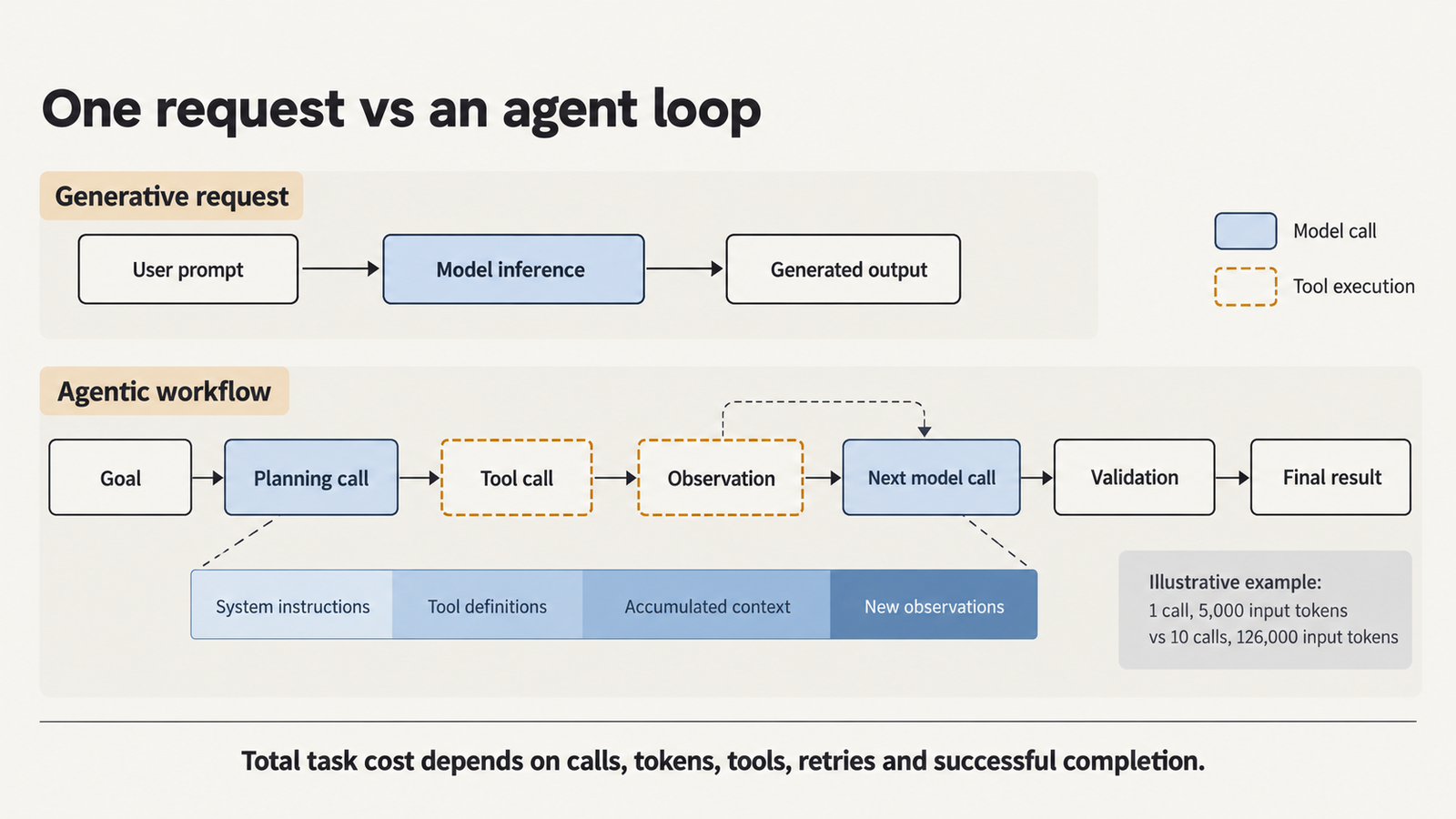
agentic AI vs generative AI

Agentic AI vs generative AI: the cost of completing a task

Price per million tokens tells you what a call costs, not what finished work costs, because failed attempts are paid for too.

Cost per successful task = (inference + tools + infrastructure + retries)
                           ÷ successfully completed tasks

Take a hypothetical pair using the same token assumptions, plus $0.02 per attempt for tool APIs and sandbox compute. Model A costs $1 input and $5 output per million tokens, averages 18 calls and completes 60% of tasks. Model B costs $3 and $15, averages 10 calls and completes 92%.

Per 1,000 attemptsModel AModel B
Input tokens per attempt356,400126,000
Total cost$405.90$450.50
Successful tasks600920
Cost per successful task$0.677$0.490

Model A charges a third of the token price yet costs about 38% more per completed task. Longer loops absorb most of its price advantage, and the lower completion rate does the rest. The table also ignores the 400 failed tasks, and if a person picks those up, the labour can outweigh the inference bill. Our breakdown of the three numbers inside inference cost per token explains how list prices become the rate you actually pay.

What caching changes

Anthropic’s prompt-caching documentation, checked on 18 October 2026, prices five-minute cache writes at 1.25× the base input rate and reads at 0.1× for many models. The cache lasts five minutes by default, refreshed on each use, and changing tool definitions invalidates all of it. OpenAI’s caching guide describes automatic caching with a 1,024-token minimum and, for GPT-5.6 and later, the same 1.25× and 0.1× multipliers.

Apply those multipliers to the ten-call example, with each call reading the previous prefix and writing only its new tokens. The task falls from $0.431 to $0.162, about 62% less. If every step instead waits past the cache lifetime, perhaps for human approval, each call writes and none reads. The task then costs $0.525, about 22% more than with no caching. Measure your hit rate before counting on the discount.

Agentic AI vs generative AI when a step fails

A wrong answer and a wrong action differ mainly in what has already happened by the time anyone notices.

A generated output that’s wrongAn agent action that’s wrong
A summary misstates a contract termThe agent writes the wrong term into the contract record
A code suggestion has a destructive bugThe agent runs that code with production write access
A recommendation names the wrong supplierThe agent emails that supplier or calls its ordering API

The left column still needs a person to act. The right column doesn’t. The line isn’t absolute, though: people act on unchecked generated text, and a read-only agent may never change anything.

Errors also compound. Anthropic’s write-up says plainly, “Agents are stateful and errors compound.” If ten independent steps each succeed 95% of the time, all ten succeed only about 60% of the time (0.95¹⁰ ≈ 0.60). Real steps aren’t independent, so treat that as arithmetic, not a forecast.

Picture a refund agent whose database write commits but whose confirmation times out. A naive retry issues a second refund. The controls that contain this are:

  • Validation: code checks each proposed action against a schema and business rules before it runs.
  • Idempotency keys: a retried write applies only once.
  • Bounded retries: attempts are capped per step and per task.
  • Transaction boundaries: related writes commit together or not at all.
  • Approval gates: a person confirms costly or irreversible actions.
  • Compensation: each action that can’t be undone directly has a defined correcting action.
  • Audit logs: the system records what was proposed, what ran and under which identity.

Agentic AI vs generative AI: security is an execution problem

A model that follows instructions well still isn’t a security boundary. The OWASP Top 10 for LLM Applications 2025 lists Excessive Agency (LLM06) and traces it to “excessive functionality,” “excessive permissions” and “excessive autonomy.” Its fixes include “complete mediation,” meaning authorisation enforced in downstream systems rather than by the model.

Prompt injection is why. OWASP’s prompt-injection entry (LLM01) covers instructions hidden in web pages, files and other content an agent reads. It says “it is unclear if there are fool-proof methods of prevention.” The UK’s National Cyber Security Centre argued in December 2025 that prompt injection is not SQL injection. Its reasoning was that LLMs “do not enforce a security boundary between instructions and data inside a prompt.” It therefore recommended deterministic, non-LLM safeguards over filtering alone. In March 2026, NIST’s Center for AI Standards and Innovation reported a red-teaming competition with more than 250,000 attack attempts. At least one attack succeeded against each of the 13 frontier models tested.

Where the controls belong

A filter can lower the odds of an attack, but it can’t decide what an attack may do. A framework’s tool list only controls what the model can request. A “run_python” tool inside your application process inherits that process’s network access, files and credentials. Real isolation comes from the operating system, container or virtual machine, plus egress rules and per-tool credentials. Our guide to the four layers of sandbox isolation covers how each layer limits damage.

The controls that matter are:

  • Least privilege: each tool gets only the access its job needs.
  • Tool allowlists: the agent calls named, reviewed tools, with no general shell unless the task requires one.
  • Scoped credentials: each tool has its own short-lived token.
  • Egress restrictions: outbound traffic is blocked by default.
  • Sandboxing: generated code runs outside the application’s process.
  • Human approval: payments, deletions and external messages wait for a person.
  • Independent policy enforcement: a separate check decides whether each action is authorised.

No single item makes an agent secure. OWASP’s Top 10 for Agentic Applications (December 2025) lists Agent Goal Hijack, Tool Misuse, Identity & Privilege Abuse and Cascading Failures as separate risks. Each needs its own control.
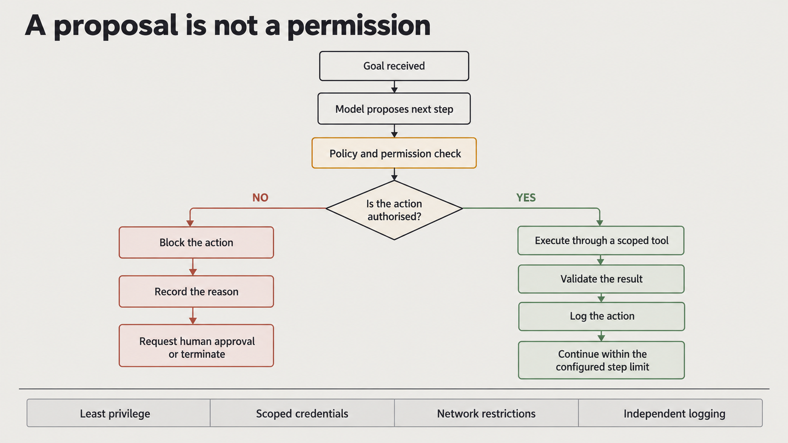
agentic AI vs generative AI

Agentic AI vs generative AI under rate limits

Four measures get confused. Requests per minute (RPM) counts API calls. Tokens per minute (TPM) counts text processed. In-flight concurrency is how many requests are open at once, and end-to-end latency is how long the user waits.

Providers measure these differently. On 18 October 2026:

  • OpenAI sets RPM, TPM and daily limits per organisation and project. Its guide warns that “unsuccessful requests contribute to your per-minute limit.”
  • Anthropic sets RPM and separate input and output TPM per model class. Its documentation says cache reads don’t count toward input limits for most models.
  • Google’s Gemini API applies RPM, TPM and daily limits per project, not per key, and says they “are not guaranteed.”
An illustrative fan-out

Suppose 100 users start a task in the same minute, using the five-call agent above. Each of its four tool steps runs three tools in parallel. Each model call takes 6 seconds and each tool step 2 seconds.

In that minuteSingle callFive-call agent
Model requests100500
Input tokens500,0004,050,000
Downstream tool calls01,200
Time per taskabout 6 secondsabout 38 seconds

The agent sends five times the requests and about eight times the input tokens, and it also loads your own systems, such as a search API or CRM. With caching on a provider that excludes cache reads, the input counted against limits drops to about 1.17 million, but the request count doesn’t change.

Retries can make this worse, because immediate retries after 429 errors add requests to a minute that’s already full. Honour any retry-after header, and otherwise use exponential backoff with random jitter, which Marc Brooker’s AWS analysis showed cuts wasted work sharply. Agents also need bounded concurrency per model and tool, a queue that holds new tasks instead of failing them, cancellation of abandoned branches, and hard caps on steps, time and tokens. Our reference on AI API rate limits in 2026 compares each provider’s published ceilings.

When a pipeline beats an agent

Anthropic’s advice is to find “the simplest solution possible,” because agentic systems “trade latency and cost for better task performance.” That trade only pays when you need the performance.

A deterministic pipeline is the better choice when you can list the steps in advance, check each output in code, run at high volume, or meet a tight latency budget. Pipelines still use generative models: one call classifies a ticket, another extracts fields, and a third drafts the reply, with code fixing the order.

Agents earn their cost when the next step depends on what the last one found, as in debugging or open-ended research. Even then, a bounded agent often works best. It has narrow tools, a step limit and deterministic checks before any write, and it sits inside a larger pipeline.

A practical decision table

ScenarioLikely architectureWhy it fitsMain concern
Single-turn drafting and summarisationOne model callThe output is the product, and a person reviews itAccuracy
Structured extraction and classificationPipeline with schema validationFixed steps; output checkable in codeSilent field errors at volume
Research across several sourcesBounded agent with read-only toolsThe next search depends on the last resultToken growth; injected content
Database updates and external transactionsPipeline, or an agent that only proposes, with approval and idempotent writesSide effects must be validated and reversibleDuplicate or unauthorised writes
Long-running multi-step workflowsWorkflow engine with agent steps insideState and retries belong in infrastructureCache expiry, lost state, runaway loops
High-volume, latency-sensitive requestsSingle call or short fixed chainPredictable latency and limitsFan-out and retries under load

Conclusion

The difference between agentic AI and generative AI shows up in operations more than output. An agent multiplies calls, compounds errors, holds permissions and loads rate limits in ways a single generation doesn’t.

So use one model call when one output answers the request, and a pipeline when you can write down the steps. Use an agent only when the next step depends on what the last one found. Then give it a step limit, a token budget, scoped credentials and a checker that isn’t the model.

FAQ

What is the difference between agentic AI and generative AI?

Generative AI produces content from a prompt. Agentic AI is a system that pursues a goal over several steps, choosing actions, calling tools and using the results. Agents usually rely on a generative model to decide.

Can generative AI become part of an agentic system?

Yes, and it usually does. The model plans, picks tools and writes the answer, while the application runs the loop, executes tools and enforces limits.

Is agentic AI more expensive than generative AI?

Usually, per task, because one task triggers many calls that re-send context. Caching, state management and completion rate can matter more than token price.

Is agentic AI more dangerous than generative AI?

Its risks are different. An agent can act without a person in between, so mistakes and injected instructions can have direct effects. The risk scales with the permissions the system grants.

When should a company use a deterministic workflow instead of an AI agent?

Use one when the steps are known in advance, outputs can be checked in code, or volume and latency demands are high. Use an agent when the path truly depends on intermediate results.

How do you measure the cost of an agentic AI task?

Divide total inference, tool, infrastructure and retry costs by the number of successfully completed tasks. Track calls per task, tokens per call, cache hit rate and completion rate separately.

How can developers limit an AI agent’s permissions and actions?

Give each tool scoped, short-lived credentials, and run generated code in a sandbox with outbound traffic blocked by default. Require human approval for consequential actions, enforce authorisation outside the model, and cap steps, time and tokens.


Keep reading

Kimi K3.1 Pro

Kimi K3.1 Pro vs Sonnet 5.5: Same Price, Different Bill

On paper, Moonshot AI priced Kimi K3.1 Pro to the cent against Claude Sonnet 5.5: $2 per million input tokens and $10 per million output …
RAG vs fine-tuning

RAG vs Fine-Tuning: Which One You Actually Need
Take a support team that ships two prototypes on the same base model. The first searches the product documentation on every question and pastes the …
AI capex

AI Infrastructure Spending: What $145 Billion and a Sold-Out AWS Actually Buy

Published 25 October 2026 · Last verified 25 October 2026 · By the UniverseBlend editorial desk On 21 October, Meta set the latest marker for …
agentic AI

What Is Agentic AI? How AI Agents Work, What They Cost, and Where They Fail

Agentic AI describes software systems in which a language model chooses and carries out a sequence of actions to complete a task. It calls tools, …

Announced vs Delivered Megawatts: Data Centre Capacity Delivery

data centre capacity delivery

Bloomberg reported on 15 October that Nscale’s flagship data centre at Glomfjord, just north of the Arctic Circle in Norway, was running about six months behind schedule. Only 6.4 MW of a planned 30 MW were in operation, according to accounts of the report. The timing matters. A month earlier, the British neocloud had filed to list on the New York Stock Exchange, reportedly targeting a valuation of up to $35 billion. Its filing showed $103.4 billion of contracted value, of which only $2.6 billion was active. Data centre capacity delivery, the slow conversion of announced megawatts into compute that customers use and pay for, is the variable underneath that gap. The industry routinely reports it as if it were a single number.

Key Takeaways
  • The reported numbers give 21.3%, not a completion rate. 6.4 MW running against 30 MW planned is 21.3% of the plan, or a 23.6 MW difference. Neither figure’s definition has been published, so that’s arithmetic, not a progress score.
  • The site’s customer is ByteDance, not Microsoft. Reports citing Bloomberg say Glomfjord is being built for ByteDance. Microsoft’s contracted Norway capacity is at a separate Narvik site due in 2027.
  • Nscale’s own figures disagree. The company’s website lists Glomfjord as “30 MW operational.” Bloomberg reports 6.4 MW running. Both can be true only if they measure different things.
  • Contract value runs well ahead of active revenue. Nscale’s filing shows $2.6 billion active out of $103.4 billion contracted, and about 25,000 active GPUs out of 461,000 active or contracted.
  • Delay costs money before it costs revenue. Bloomberg reports penalties of millions of dollars, settled with better terms on new contracts. The filing lets Anthropic cancel tranches delivered too late.
  • Capacity should be reported by milestone. Announced, energised, commissioned, accepted and serving workloads are different facts, and investors need each one stated separately.

Quick Navigation


Two numbers that don’t measure the same thing

Start with the arithmetic, because it is the only part that can be stated with certainty. 6.4 divided by 30 is 21.3%. The difference is 23.6 MW. What those numbers mean is harder to say.

Bloomberg’s report, as relayed by Quartz and DCD, describes 30 MW as planned and 6.4 MW as running. It doesn’t say whether either figure is IT load (power available to servers), total facility power including cooling, or grid connection capacity. These can differ substantially. A site with a 30 MW grid connection may support noticeably less IT load once cooling and electrical losses are counted.

The company’s own description adds to the confusion. Nscale’s Glomfjord page lists the site as “30 MW operational” and “expandable to 60 MW.” In March 2025, DCD reported that Nscale and InfraPartners would add a 30 MW liquid-cooled building next to the existing 30 MW, set to “go live in Q2 2025.” One plausible reading is that Bloomberg’s planned 30 MW refers to that new building rather than the whole campus. If so, an older facility is operating alongside it. That would make the 21.3% a measure of the expansion only. We couldn’t confirm it, and Nscale declined to comment to Bloomberg, citing its pre-IPO quiet period.

The customer is also different from what’s often assumed. Microsoft is Nscale’s biggest contracted customer overall: its agreements provide for payments of up to about $43.8 billion through December 2033, according to the filing as reported by TokenPost. But reports citing Bloomberg say Glomfjord is being built for ByteDance. Tom’s Hardware found that a ByteDance subsidiary, Spring (SG), accounted for 73% of Nscale’s 2025 revenue through 2,304 Nvidia B200 GPUs at the site. Microsoft’s Norway capacity is at Narvik, a 230 MW joint-venture site with Aker that is due to deliver in 2027.

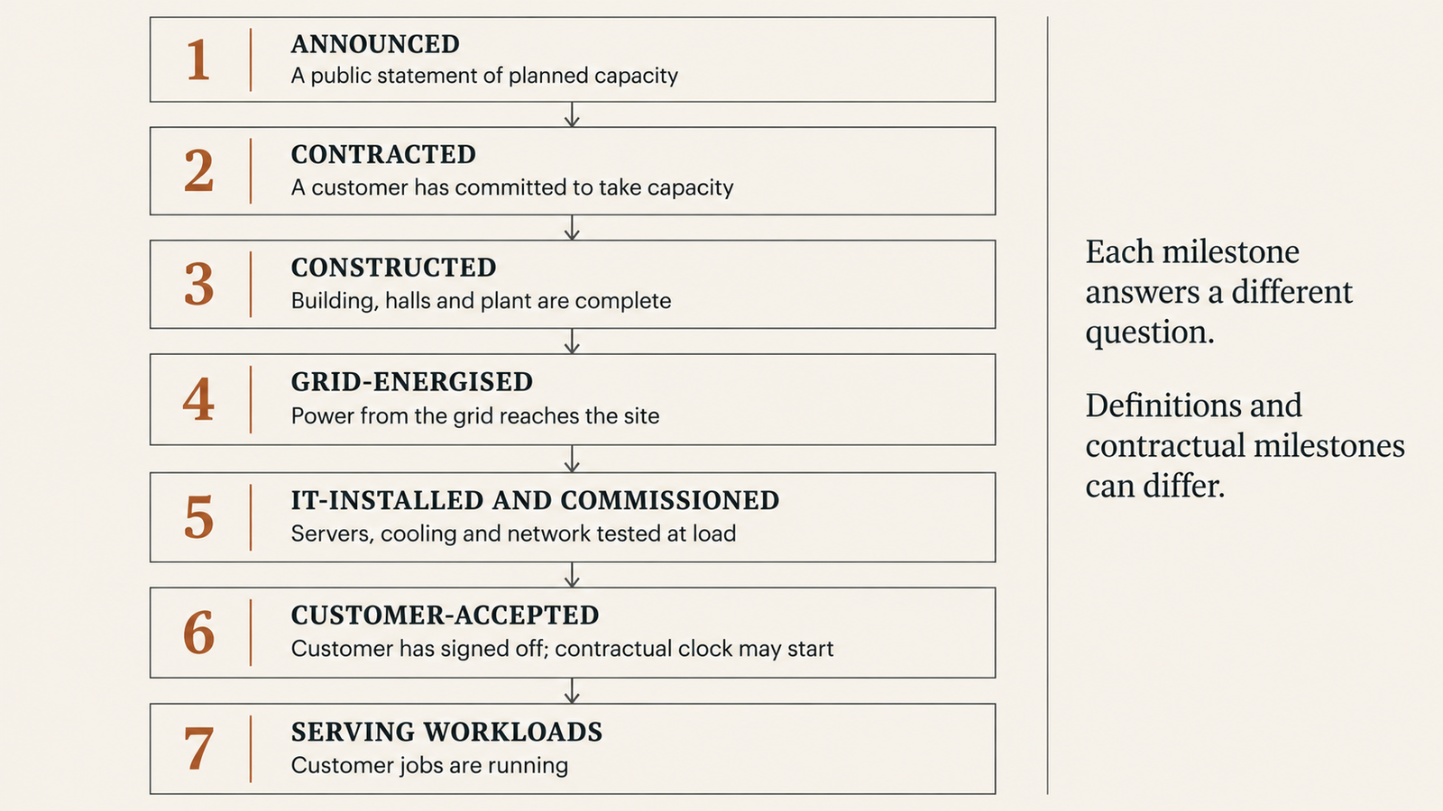
A seven-step audit of data centre capacity delivery

A megawatt passes through several states before it earns money, and announcements rarely say which one they mean. The seven below aren’t a universal sequence. Contracts can define delivery differently from engineering milestones, and large sites are commissioned in phases. Still, each state answers a different question.

StageWhat it meansThe question it answers
AnnouncedA public statement of planned capacityWhat does the company intend to build?
ContractedA customer has committed to take capacity on agreed termsWho has agreed to pay, and when?
ConstructedBuilding shell, halls and plant are physically completeDoes the facility exist?
EnergisedThe grid connection is live and power reaches the site’s distributionCan the site draw its rated power?
Installed and commissionedServers, accelerators, networking and cooling are installed and tested togetherCan the equipment run at load?
Customer-acceptedThe customer has signed off against contractual testsHas billing, or the contractual clock, started?
Serving workloadsCustomer jobs are runningIs the capacity doing useful work?

The gap between stages 1 and 7 is where pipelines start to look different from reality. Nscale’s filing illustrates the scale: about 25,000 GPUs active out of 461,000 classified as active or contracted. That’s not evidence of anything going wrong. Most of those contracts are for capacity that was never meant to exist yet. But a headline figure that blends all seven stages tells an investor very little about near-term revenue.

data centre capacity delivery

The physical chain behind data centre capacity delivery

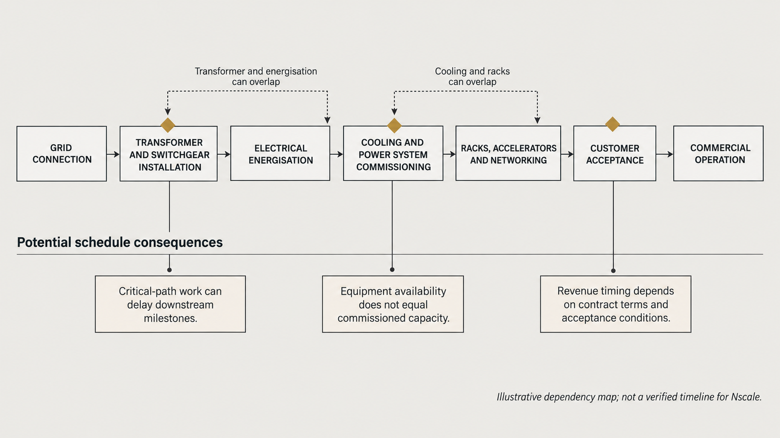
Behind every operational megawatt is a chain of dependencies, and a hold-up in one link stops everything after it. The chain runs roughly like this. A grid connection has to be agreed and the network reinforced. High-voltage transformers and switchgear have to be delivered, installed and protected. The building and its cooling and power distribution have to be finished and commissioned. Only then can racks, accelerators and network fabric be installed, tested and handed to a customer.

At Glomfjord, Bloomberg’s reporting points to problems in the middle of that chain, not at the grid connection. According to Quartz’s account, Bloomberg cited slow construction, local regulatory hurdles and coolant leaks. It also cited a fire that began in December when a transformer burned, which Bloomberg drew from public records. A Norwegian safety agency identified 10 violations at the site, and regulators closed the case in September after Nscale made fixes. DCD adds that Nscale towed in a floating hotel, the Kalmar, to house construction workers.

That list establishes what went wrong at this site. It doesn’t establish how much each problem contributed to the six months. A transformer fire is a specific event. That doesn’t make it a sign of the industry-wide transformer shortage that often features in reporting on data centre delays, and nothing in the public record links Glomfjord’s delay to equipment lead times or grid capacity. Likewise, coolant leaks in a liquid-cooled hall are a commissioning failure. They aren’t evidence that liquid cooling is unworkable.

The last stage of the chain is the least visible. A hall can be energised and cooled with its GPUs on site and still not serve a customer. Racks need integrating, the network fabric has to be built and tested, firmware and drivers have to be aligned, and the customer’s acceptance tests have to pass. Even then, the hardware has to be kept busy. As our analysis of why accelerator utilisation decides the cost of every token argued, idle accelerators still have to be paid for. A commissioned megawatt with low utilisation costs much the same and earns far less.

data centre capacity delivery

The Arctic trade-off at Glomfjord

The case for building near the Arctic Circle is real but specific. Nscale says the site runs on “100% renewable power generated by the region’s hydropower dams,” uses adiabatic cooling that “leverages the local climate,” and benefits from a “stable oversupply” of renewable power. These are the company’s claims. The low ambient temperatures are a matter of geography. The power claims haven’t been independently tested in public, and the grid-oversupply claim comes with no figures.

The costs are specific too. Nscale’s own site page describes Glomfjord as “a small industrial town of 1000 people.” A town that size has limited local workforce, accommodation and contractor capacity for a fast build, which is consistent with the reported need to bring in a floating hotel for workers. Specialist equipment and replacement parts have to travel further, and replacing a failed transformer can take longer far from major suppliers. None of this proves that the location caused the delay. It does mean that the conditions that make Glomfjord efficient to run are different from the ones that make it fast to build.

The general lesson is narrower than “Nordic sites are slow.” Cheap, clean power and cold air reduce operating costs once a site is running. They do little to speed up construction, and they can’t make a remote site easier to staff. A buyer comparing sites needs both numbers: the operating cost per megawatt and the date by which that megawatt will be delivered.

Stress-testing the revenue timeline

A delay doesn’t just postpone revenue. It changes when each cash flow happens, and those changes don’t move in step.

Four events are often treated as one: accounting revenue recognition, contractual payment obligations, cash collection, and actual workload consumption. Under many capacity contracts, the customer’s obligation starts at acceptance, not at energisation. Revenue is then recognised as capacity is made available, cash arrives on the invoice terms, and the customer’s workloads may ramp up more slowly than either. Nscale’s Glomfjord contract terms aren’t public, so it’s unknown which of these the delay pushed back, or by how much.

What the filing does disclose is that the risk runs both ways. Nscale says its contracts include delivery milestones, service-level requirements and penalties for delay. Anthropic may terminate a tranche without liability if Nscale fails to deliver it within a specified period after the expected delivery date. Bloomberg reported, through people familiar with the matter, that Glomfjord’s delays left Nscale liable for penalties totalling millions of dollars. Customers were reportedly offered better terms on new contracts instead of collecting them. That’s a quieter cost, but a real one. It shows up as lower future margins, not as a one-off charge.

Here’s an illustrative calculation. It isn’t Nscale’s data. Suppose a provider spends $1 billion building and equipping a hall that is expected to bill $20 million a month from acceptance. A six-month delay defers $120 million of billings, but the capital is already spent and financing costs keep running. At an 8% annual cost of debt on the full $1 billion, six months of interest is about $40 million. That’s money paid with nothing coming in, before any penalties or concessions. The figures are hypothetical. The mechanism isn’t. Capex goes out on the construction timeline, and income arrives on the acceptance timeline.

That mechanism is why delivery risk reaches the balance sheet. Our analysis of how lenders repriced CoreWeave’s AI infrastructure debt found the same gap at a much larger scale. CoreWeave’s $103.7 billion of remaining performance obligations depended on capacity that hadn’t yet been built, while its debt payments were already scheduled. Nscale’s $103.4 billion contract figure is a different measure from CoreWeave’s RPO, but the same question applies to both: how much of it can be delivered before the bills come due?

Reading a capacity pipeline before an IPO

Pipeline figures are hard to compare because they measure different things, and press releases rarely say which. Three recent examples show the range.

Google’s 6 October agreements with Constellation, reported as 3.59 GW, are electricity supply: an 890 MW, 20-year nuclear-uprate power purchase agreement and a 2,700 MW, 15-year supply deal. That’s power secured, not data-centre capacity built. Alibaba’s 20 GW is a stated target for Alibaba Cloud’s data-centre capacity by 2032. It’s stage 1 in the audit above. Nscale’s $103.4 billion is contracted value, measured in dollars rather than megawatts. Adding or ranking these figures against each other would produce a meaningless number.

The same caution applies to compute commitments. As we found in our analysis of the obligation behind Anthropic’s $518 billion compute commitment, a commitment from the buyer’s side depends on capacity that providers like Nscale still have to deliver. A delay at the supplier becomes a timing problem for the buyer.

For anyone reading a prospectus, a short set of questions separates pipeline from production:

  • Which measure? IT load, facility power or grid connection, and is it stated as nameplate or delivered?
  • Which stage? Contracted, energised, commissioned, accepted or serving workloads. How much is at each stage today?
  • When does the money start? At delivery, acceptance or consumption, and what penalties or termination rights apply if the date slips?
  • What’s the conversion record? How have previous sites performed against their announced dates and capacities?
  • Who carries the gap? Is construction financing committed, or does it depend on a capital raise that a delay could make harder?

The last point applies here. Nscale’s filing says it had no binding financing commitments for the Anthropic agreements, which are its largest. That doesn’t mean it can’t get financing. It does mean the delivery timeline and the financing timeline depend on each other.

What data centre capacity delivery reporting should look like

The Glomfjord reports don’t show that Nscale’s business model is broken. A delay of six months at one site, with fires, leaks and inspections along the way, is the kind of thing that happens on complex industrial projects, and a delay isn’t a failure. What the episode shows is how little a single headline megawatt figure tells you. The same campus is “30 MW operational” on the company’s website and 6.4 MW running in Bloomberg’s reporting, and readers can’t tell which figure describes what.

A better standard would be simple: report capacity at each milestone, define the unit used, and give the date. Announced, energised, commissioned, accepted and serving workloads are five different facts. A company preparing to list at a reported valuation of up to $35 billion is better served by publishing all five than by asking investors to trust one. Until the industry reports data centre capacity delivery that way, the gap between announced and delivered megawatts will keep turning up in places like Glomfjord, and readers will find out about it from news reports rather than from the companies.

FAQ

What is the difference between announced and operational data centre capacity?

Announced capacity is what a company plans or has publicly committed to build. Operational capacity is what is energised, commissioned and running workloads. Between the two are construction, grid connection, equipment installation and customer acceptance, and any of them can slip.

Why are data centre projects delayed after they’re announced?

Common causes include grid connection and network reinforcement, delivery and installation of transformers and switchgear, construction and permitting, cooling and power commissioning, and integrating servers and networks. At Glomfjord, Bloomberg reported slow construction, regulation, coolant leaks and a transformer fire. It didn’t say how much each contributed.

How does grid energisation differ from commissioning?

Energisation means the grid connection is live and power can reach the site. Commissioning means the site’s cooling, electrical systems and IT equipment have been tested together at load. A site can be energised long before it is commissioned.

What does a delayed data centre mean for revenue?

It usually defers billing, which often starts at customer acceptance, while construction and financing costs continue. It can also trigger penalties or contract concessions. The exact effect depends on contract terms, which are rarely public.

How should investors read a contracted capacity pipeline?

Ask what unit each figure uses, which milestone it has reached, when payments start, what happens if delivery slips, and how the company’s past sites performed against their announced schedules. Nscale’s filing shows $2.6 billion active out of $103.4 billion contracted, a ratio worth asking about.


Keep reading

Kimi K3.1 Pro

Kimi K3.1 Pro vs Sonnet 5.5: Same Price, Different Bill

On paper, Moonshot AI priced Kimi K3.1 Pro to the cent against Claude Sonnet 5.5: $2 per million input tokens and $10 per million output …
RAG vs fine-tuning

RAG vs Fine-Tuning: Which One You Actually Need

Take a support team that ships two prototypes on the same base model. The first searches the product documentation on every question and pastes the …
AI capex

AI Infrastructure Spending: What $145 Billion and a Sold-Out AWS Actually Buy
Published 25 October 2026 · Last verified 25 October 2026 · By the UniverseBlend editorial desk On 21 October, Meta set the latest marker for …
agentic AI

What Is Agentic AI? How AI Agents Work, What They Cost, and Where They Fail

Agentic AI describes software systems in which a language model chooses and carries out a sequence of actions to complete a task. It calls tools, …

When Adding an Agent Stops Paying for Itself

multi-agent token cost

The architecture that became more expensive without becoming better

Multi-agent token cost rarely shows up in a design review. It shows up a month later on the invoice. Take a team that splits a defect-investigation agent into a planner, three specialist workers and a synthesiser. Its fix rate improves, so it scales to eight workers. The fix rate stays flat and the per-run model bill more than doubles.

Nothing went wrong with the models. Each worker reread the same code, wrote its own notes, and handed them to a synthesiser that read them all again. Per-token prices have fallen over the past year, but this system now buys far more tokens per answer. A cheaper token and a more expensive system can coexist, and that gap is the subject of this article.

Key Takeaways
  • Agent count is a poor proxy for quality. In the largest controlled study available, multi-agent setups averaged −0.3% against a single agent, with results ranging from +80.8% to −70% depending on the task.
  • Most extra tokens come from repeated context. In this article’s eight-agent example, workers rereading the same 20,000-token code context account for 72% of all input tokens.
  • In the example, going from one to three agents cost $2.34 per additional successful task. Going from three to five cost $12.95. Going from five to eight cost $0.78 more per run with no gain.
  • Token prices and GPU rental prices are separate markets. Falling API rates do not mean falling H100 rents, and the dated data does not show that they have.
  • Extra agents can still pay when subtasks are genuinely independent, when a failure is expensive, or when parallel work cuts latency someone cares about.
  • Before adding an agent, run an ablation. Remove it, rerun the same evaluation set, and compare cost per successful task.

Quick Navigation


The multi-agent token cost is hidden in the handoffs

Agents are not the unit of cost. Model calls are, and every call pays for its whole input again.

A single agent investigating a bug might make eight calls. It starts with the bug report and the relevant code, about 20,000 tokens, and appends what it learns as it goes. By the last call its input is larger, but it only ever pays for one copy of the codebase per call.

Split that work across workers and the arithmetic changes. A planner reads the task and writes assignments. Each worker then reads the same code plus its own brief, makes a few calls of its own, and writes a report. A synthesiser reads every report alongside the original context. The code that the single agent read eight times is now read four times per worker, by every worker.

That is the first cost driver: duplicated context. The second is intermediate output. Plans, reports and summaries are output tokens, billed at five times the input rate on many current models, and then billed again as input when the next agent reads them. Retries add a third layer. A worker that fails a tool call reruns with its full context.

None of this makes multi-agent design wrong. It means the useful question is how much an added worker contributes beyond the context it rebuys, not how many agents a system has. UniverseBlend found the same pattern in a different form in its analysis of why a 50% price cut doesn’t halve agent bills: in agent workloads, the line item that repeats matters more than the headline rate.

What the research on multi-agent scaling establishes

The circulating claim that agent quality plateaus while token use keeps climbing has a real basis, but not a single magic number behind it. No paper dated October 12, 2026 matching that claim could be found. The strongest primary evidence is earlier and more careful.

Kim and colleagues at Google Research, Google DeepMind and MIT tested 260 configurations in Towards a Science of Scaling Agent Systems (arXiv, version 3 dated April 8, 2026). They compared a single agent against four multi-agent designs across six agentic benchmarks, from financial analysis to SWE-bench Verified, using OpenAI, Google and Anthropic models.

The headline is variance, not improvement. Averaged across every multi-agent result, performance changed by −0.3% relative to a single agent, with a 95% interval running from −58.7% to +77.2%. A centralised design improved Finance-Agent by 80.8%. Every multi-agent design made PlanCraft worse, by 39.1% to 70.0%. On SWE-bench Verified, all variants lost ground.

Two findings bear directly on cost. First, token efficiency collapsed. A single agent produced 67.7 successes per thousand tokens; centralised and hybrid teams produced 21.5 and 13.6. Second, tasks where a single agent already scored above 45% saw negative returns from adding agents. This was the paper’s most statistically robust result (β = −0.236, p = 0.004).

The agent-count question itself was a smaller, preliminary test. Using Gemini models at 1, 3, 5, 7 and 9 agents, the authors report that Gemini 2.0 Flash peaked at seven agents before degrading, and that a centralised Gemini 2.5 Pro team showed diminishing returns beyond five. The paper does not give the exact accuracies or name the benchmark for that figure. So “quality plateaus at five agents” is too strong a summary. The defensible reading is that the optimum depends on model and coordination design, and it arrived at single-digit team sizes in the cases tested.

The study did not measure latency, and it reports dollar cost only as marginal cost per point of success for one architecture. A newer paper on vulnerability-discovery agents, Where Do the Tokens Go? (October 8, 2026), adds a consistent observation from a different domain: “higher spending does not consistently yield better outcomes.” It does not vary agent count, so it supports the spending point and nothing more.

The practical consequence is that there is no published universal agent count to copy. Each team has to measure its own curve.

The four-configuration multi-agent token cost test

What follows is a transparent cost model, not a benchmark. Token counts and success rates are illustrative assumptions chosen to be plausible and consistent with the research above. Prices are real.

  • Task (same for all four): investigate a reported defect in a service and produce a root cause plus a proposed patch. Success means the patch passes the project’s existing test suite and a reviewer accepts the diagnosis.
  • Model and prices: Claude Sonnet 5.5, $2.00 per million input tokens and $10.00 per million output tokens, USD, from Anthropic’s pricing page, checked October 11, 2026.
  • Included: every priced model call (planner, workers, synthesiser).
  • Excluded: prompt caching, retries, tool execution, embeddings, external search, orchestration servers and engineering time.

Workload assumptions:

  • Shared context: 20,000 tokens (bug report plus relevant code).
  • One agent: 8 sequential calls, average input 32,000 tokens (shared context plus 12,000 accumulated notes), 1,500 output tokens each.
  • Multi-agent (n workers): one planner call (21,000 in / 2,000 out); each worker makes 4 calls averaging 26,000 input (shared context, brief and own notes) and 1,200 output; one synthesiser call reading the shared context, a 1,500-token report per worker and the 2,000-token plan, writing 3,000 tokens.
  • Success rates (illustrative): 38%, 50%, 54% and 53%. The single-agent baseline is set below the 45% level at which Kim et al. found extra agents start to hurt. The slight drop at eight reflects the degradation they observed at larger team sizes.
Token arithmetic
  • 1 agent: input 8 × 32,000 = 256,000; output 8 × 1,500 = 12,000.
  • 3 agents: input 21,000 + (3 × 4 × 26,000 = 312,000) + (20,000 + 4,500 + 2,000 = 26,500) = 359,500; output 2,000 + 14,400 + 3,000 = 19,400.
  • 5 agents: input 21,000 + 520,000 + 29,500 = 570,500; output 2,000 + 24,000 + 3,000 = 29,000.
  • 8 agents: input 21,000 + 832,000 + 34,000 = 887,000; output 2,000 + 38,400 + 3,000 = 43,400.

Cost = input tokens ÷ 1,000,000 × $2.00 + output tokens ÷ 1,000,000 × $10.00.

Results
Metric1 agent3 agents5 agents8 agents
Input tokens256,000359,500570,500887,000
Output tokens12,00019,40029,00043,400
Total tokens268,000378,900599,500930,400
Input cost$0.512$0.719$1.141$1.774
Output cost$0.120$0.194$0.290$0.434
Total API cost per run$0.632$0.913$1.431$2.208
Success rate (illustrative)38%50%54%53%
Incremental cost vs previous—+$0.281+$0.518+$0.777
Incremental success vs previous—+12 pts+4 pts−1 pt
Cost per successful task$1.66$1.83$2.65$4.17
Latency (estimate, 8 s per call, workers fully parallel)~64 s~48 s~48 s~48 s
multi-agent token cost

These are four different measurements. Total tokens tripled between one and five agents (268,000 to 599,500), while cost per successful task rose by 60% ($1.66 to $2.65). The ratios differ because more successes partly offset the extra spend. Latency improves when workers run in parallel, as long as the provider lets eight 26,000-token requests run at once. That depends on tokens-per-minute limits, covered in UniverseBlend’s guide to AI API rate limits in 2026. The latency figures are illustrative too.

The point where more agents stop paying

The marginal numbers carry the argument.

  • One to three agents: +$0.281 per run for +12 points of success, or $0.281 ÷ 0.12 = $2.34 per additional successful task.
  • Three to five: +$0.518 for +4 points = $12.95 per additional success.
  • Five to eight: +$0.777 for −1 point. No additional successes, so the move never pays.

Whether $12.95 is too much depends on what a success is worth, which the token bill cannot tell you. The rule is to add the agent only if (gain in success rate) × (value of one success) is greater than the added cost per run.

If a resolved defect saves an engineer an hour, valued at $50, then 0.04 × $50 = $2.00 exceeds $0.518 and five agents beat three. If the task is low-stakes triage worth $5 per success, 0.04 × $5 = $0.20 falls short, and three agents is the right stopping point. Eight agents lose at any value, because they produce no gain.

That is the honest answer to the headline. In this example the agent stops paying for itself at the configuration where its marginal success gain, times what a success is worth, drops below its marginal tokens. The break-even depends on the value of a success, not on a universal number of agents.

Four task properties move that point.

  1. Independence of subtasks. Workers that split a search space with little overlap add coverage cheaply. Workers that all need the full context mostly add duplicated reading. That is the Finance-Agent pattern versus the PlanCraft pattern in Kim et al.
  2. Baseline strength. When a single agent already succeeds most of the time, there is little left to gain and more room for coordination errors.
  3. Error propagation. Kim et al. measured error amplification of 17.2× for independent agents against 4.4× for centralised designs with a verifier. More agents without a checking step multiply mistakes as well as tokens.
  4. Cost of failure. For security review, financial reconciliation or production incidents, a second independent opinion can be worth many times its tokens even at a small success gain.

Why cheaper tokens do not guarantee cheaper AI systems

API prices have fallen. OpenAI’s GPT-6 Sol launched at $2 input and $10 output per million tokens, half the $4 and $20 of GPT-5.6 Sol, as UniverseBlend covered in September. On the current model page, GPT-6.1 Sol still lists $2 and $10.

GPU rents have not followed. The Silicon Data H100 rental index read $2.85 per GPU-hour on October 12, 2026, up 1.1% over the previous week. SemiAnalysis has reported one-year H100 rentals rising from about $1.70 in October 2025 to about $2.35 in March 2026. That figure could not be independently opened for this article and should be treated as reported, not verified. On-demand list prices on October 10 still ran from $2.89 to $11.68 per GPU-hour depending on provider and configuration, as tracked in UniverseBlend’s GPU cloud pricing comparison.

The two prices measure different things. An API price is what a provider charges per token, after its own hardware efficiency, batching and margin. A GPU rent is what scarce hardware fetches by the hour. Better software, quantisation and newer chips can push the token price down while demand for the hardware pushes its rent up. Both can be true at once without contradicting each other.

This is where Jevons’ paradox gets invoked. William Stanley Jevons observed in The Coal Question (1865) that more efficient steam engines increased Britain’s total coal consumption, because cheaper effective energy opened new uses. The AI version says cheaper tokens unlock workloads, multi-agent systems among them, that consume so many more tokens that total compute demand rises.

The analogy needs conditions before it holds. Demand for tokens must be elastic enough that lower prices raise total spending, not just volume. The efficiency gain must be what lowered the price, not a subsidy or promotional pricing. And the measure must be total resource use, not one company’s bill. The dated evidence here shows falling list prices and stable-to-rising GPU rents. That is consistent with Jevons, but it does not prove it. Supply constraints alone could explain firm rents.

For a team running agents, the practical point is narrower. A cheaper model makes each token cheaper, but an architecture that multiplies tokens 3.5-fold, as eight agents did in the example, can absorb a 50% price cut and still cost more. If you self-host, the relevant price is the GPU-hour and your utilisation, not the API rate card.

A decision rule engineers can actually use

Add an agent only when its measured marginal contribution is worth its marginal cost:

\Delta p \times V_{\text{success}} \; > \; \Delta C_{\text{run}} + \Delta C_{\text{latency}} + \Delta C_{\text{operations}}

Here Δp is the change in success rate, V is the value of one success, and the right side is the added cost per run in tokens, waiting time and operational burden.

Before adding one, check:

  • Baseline quality: what does the simplest configuration achieve on a fixed evaluation set?
  • Incremental success: how much does the new agent change the success rate, with confidence intervals?
  • Added tokens: how many input and output tokens does it add per run, including the context it rereads?
  • Marginal cost: what is the cost per additional successful task?
  • Latency: does it shorten or lengthen end-to-end time at your rate limits?
  • Failure severity: what does one wrong answer cost downstream?
  • Evaluation reliability: is the evaluation set large enough to detect a gain this size?
  • Simpler alternatives: would a better prompt, a verifier step or a stronger single model do the same?

The most useful test is an ablation. Disable one agent, rerun the same evaluation set, and compare cost per successful task. If nothing measurable changes, the agent was decoration.

multi-agent token cost

What to measure before scaling the agent count

Log tokens per call, not per run, tagged with agent role, so duplicated context is visible. Track cost per successful task as the primary metric, alongside success rate, p50 and p95 latency, retries and tool-call count.

Keep offline and production numbers apart. An evaluation set measures capability on known tasks. Production traffic adds longer contexts, rate-limit queueing and failure modes the evaluation set never contained. Re-check the ablation on a production sample before committing.

Prompt caching changes the arithmetic for the duplicated-context problem specifically. If workers share an identical prefix, cache reads can cut the cost of rereading it sharply. Rerun the cost model with your actual cache-hit rate before deciding, because it can move the break-even point.

Conclusion: optimise the work, not the agent count

The evidence does not support a universal team size, and it does not support the idea that more agents are better. The largest controlled study found an average effect near zero, wide variation by task, and token efficiency falling by a factor of three or more. The worked example shows how that looks on an invoice. The first two extra agents earned their keep, the next two did so only for valuable tasks, and the last three added nothing.

Multi-agent token cost is a design variable, not a fixed tax. Split work where subtasks are genuinely independent, add verification where errors are expensive, and stop when the next agent’s marginal success, times what a success is worth, no longer covers its marginal tokens. An additional agent is justified when its measurable contribution exceeds what it costs. Nothing else about it matters.

Frequently Asked Questions

What is multi-agent token cost?

Multi-agent token cost is the total model spend of a system where several LLM agents collaborate on one task. It includes each agent’s own calls, the context every agent rereads, plans and reports passed between agents, and the final synthesis. It usually grows faster than the number of agents because shared context is paid for repeatedly.

How many agents should an AI system use?

No study supports a universal number. Kim et al. found optimal team sizes depended on the model and coordination design, with diminishing returns appearing beyond five to seven agents in their preliminary Gemini tests. Start with one agent, add one at a time, and keep each only if it improves cost per successful task.

Why do multi-agent systems consume more tokens?

Each agent rereads shared context, writes intermediate plans or reports, and passes them on to be read again. Coordination also adds turns: Kim et al. measured hybrid designs taking 44.3 turns on average against 7.2 for a single agent. Retries and synthesis calls add further tokens.

Does adding more agents improve LLM accuracy?

Sometimes. Across 260 configurations, Kim et al. found a mean change of −0.3%, with gains up to +80.8% on a financial-analysis benchmark and losses up to −70% on a planning benchmark. Tasks where a single agent already exceeded 45% accuracy tended to get worse with more agents.

How can engineers calculate cost per successful AI task?

Add up input and output token costs for every model call in a run, then divide by the run’s success rate on a fixed evaluation set. For example, $0.913 per run at 50% success is $1.83 per successful task. Compare configurations on this figure, not on raw token counts.

Does cheaper token pricing make multi-agent systems cheaper?

Only if token consumption grows more slowly than prices fall. A 50% price cut is erased by an architecture that uses 3.5 times the tokens. And for self-hosted systems, API price cuts do not lower GPU rents, which have been stable to rising in 2026.


Keep reading

Kimi K3.1 Pro

Kimi K3.1 Pro vs Sonnet 5.5: Same Price, Different Bill

On paper, Moonshot AI priced Kimi K3.1 Pro to the cent against Claude Sonnet 5.5: $2 per million input tokens and $10 per million output …
RAG vs fine-tuning

RAG vs Fine-Tuning: Which One You Actually Need

Take a support team that ships two prototypes on the same base model. The first searches the product documentation on every question and pastes the …
AI capex

AI Infrastructure Spending: What $145 Billion and a Sold-Out AWS Actually Buy
Published 25 October 2026 · Last verified 25 October 2026 · By the UniverseBlend editorial desk On 21 October, Meta set the latest marker for …
agentic AI

What Is Agentic AI? How AI Agents Work, What They Cost, and Where They Fail

Agentic AI describes software systems in which a language model chooses and carries out a sequence of actions to complete a task. It calls tools, …

LLM Context Window Comparison 2026: Limits and Costs

LLM context window

Specifications and prices checked October 11, 2026 · Prices in USD per million tokens, standard API tier

Short answer: In an LLM context window comparison for 2026, input capacity barely separates the leading models. Every proprietary API checked here accepts about 1 million tokens (1M to 1,050,000), and the two open-weight hosts list 1M or 524,288. Output caps differ more, from 65,536 tokens on Gemini to 128,000 on GPT-6.1 Sol and Claude Opus 5.5. Long-context pricing rules differ most of all: a 300,000-token prompt costs anywhere from $0.06 to $1.20 in input charges.

Three numbers get conflated in most spec sheets. The context window is how much a model can read in one request. The output limit is how much it can write back. The long-context pricing threshold is the prompt size at which the provider starts charging more. A model can have a huge window, a modest output cap and a threshold that doubles your bill well before you get near the window’s edge.

The third number is the one buyers skip. GPT-6.1 Sol charges $2.00 per million input tokens up to 272,000 tokens and $4.00 per million above it, and OpenAI applies the higher rate to the full request. A 270,000-token prompt costs $0.54. A 280,000-token prompt costs $1.12. Ten thousand extra tokens cost 58 cents.

Key Takeaways
  • Context capacity has converged. Every proprietary model checked lists about 1M input tokens, so window size rarely decides a purchase in 2026.
  • Output caps have not converged. Gemini 3.1 Pro and 3.8 Flash cap output at 65,536 tokens, about half of GPT-6.1 Sol’s and Claude Opus 5.5’s 128,000.
  • Three providers reprice by prompt size. OpenAI does it above 272K for the whole request, Google above 200K for Gemini 3.1 Pro, and Anthropic above 100K for Claude Haiku 5.5 only.
  • Claude Opus 5.5 and Sonnet 5.5 have no long-context surcharge. At 300K tokens, Opus 5.5 ($1.20) costs the same as GPT-6.1 Sol and Gemini 3.1 Pro, even though its base rate is twice theirs.
  • Crossing a threshold can cost more than the extra tokens are worth. Just past 272K, a GPT-6.1 Sol prompt more than doubles in price.
  • Caching flattens the comparison. A fully cached 300K prefix costs $0.06 on both GPT-6.1 Sol and Claude Opus 5.5.
  • Open-weight hosting is cheapest per token, but a host’s served context can differ from the model card. Check the endpoint, not the paper.

Quick Navigation


The LLM context window comparison table

All values are taken from official documentation and were checked October 11, 2026. “Threshold” is the prompt size at which input pricing changes. Costs cover input tokens only, with no output, caching, batch discounts or taxes.

Model and versionMax input contextMax outputLong-context thresholdInput belowInput above300K input costAvailabilityDocumentation
GPT-6.1 Sol (gpt-6.1-sol)1,050,000128,000>272K, whole request$2.00$4.00$1.20GA, OpenAI APIModel page
GPT-6 Luna (gpt-6-luna)1,050,000128,000>272K, whole request$0.10$0.20$0.06GA, OpenAI APIModel page
Claude Opus 5.5 (claude-opus-5-5)1M128,000None$4.00n/a$1.20Current, Claude APIModels · Pricing
Claude Sonnet 5.5 (claude-sonnet-5-5)1M128,000None$2.00n/a$0.60CurrentSame as above
Claude Haiku 5.5 (claude-haiku-5-5)1M128,000>100,000$0.10$0.50$0.15CurrentSame as above
Gemini 3.1 Pro (gemini-3.1-pro-preview)1,048,57665,536>200K$2.00$4.00$1.20PreviewModel · Pricing
Gemini 3.8 Flash (gemini-3.8-flash)1,048,57665,536None$0.75 (to Dec 31, 2026; $1.50 from Jan 1, 2027)n/a$0.225StableModel
Gemini 3.5 Flash-Lite (gemini-3.5-flash-lite)1,048,57665,536None$0.30n/a$0.09StableModel
Mistral Large 4 (mistral-large-4)1MNot publicly documentedNone documented$0.68 sale ($1.36 list)n/a$0.204 salePublic Preview, open-weightModel page
Llama 4 Maverick (Together AI)1M per model card; host lists 1,048K and 524,288Not publicly documentedNone documented$0.27n/a$0.081Hosted endpointModel card · Host
Qwen3.8-2.4T-A95B (Together AI)262,144 native; 1M served131,072None documented$2.00n/a$0.60Hosted endpointModel card · Host

Whole-request rules apply where stated. OpenAI says prompts above 272K are “priced at 2x input and cache rates and 1.5x output for the full request.” Anthropic says a Haiku 5.5 request over 100,000 tokens “pays the higher prices,” counting cache reads and writes toward prompt length. Google’s table selects the rate by prompt size (“prompts > 200k tokens”) but does not explicitly say the whole prompt is repriced. This article assumes it is, and that is an interpretation of Google’s wording.

The open-weight rows describe one host’s endpoint, not the model. Qwen3.8’s model card gives 262,144 tokens natively, extensible to about 1M. A 300K request on Together therefore runs in the extended range, where quality can differ from native-length behaviour.

Context window versus output limit

The context window caps what goes in. The output limit caps what comes out in a single response. They are documented separately for every proprietary model here, and they constrain different workloads.

Output limits bind harder than input limits. A model that reads a 400-page contract can only write 65,536 tokens back if it is Gemini 3.1 Pro, or 128,000 if it is GPT-6.1 Sol or Claude Opus 5.5. That is roughly 50,000 versus 100,000 words, before any reasoning tokens. Google bills thinking as output (“output price including thinking tokens”), so whether reasoning also draws on the output cap matters for long reasoning tasks. Check each provider’s documentation for that point, because accounting differs.

Some providers also treat input and output as one shared budget, so a large prompt leaves less room to answer. Qwen’s model card illustrates the general point: it recommends allowing 262,144 tokens for reasoning and 131,072 for the final answer, figures that only make sense if the request budget is planned as a whole.

LLM context window

Where long-context pricing start

Three of the providers checked charge more once a prompt gets long. Each draws the line in a different place and handles it a little differently.

  • OpenAI, 272K, whole request. For GPT-6.1 Sol and GPT-6 Luna, prompts above 272K input tokens pay double the input and cache rates and 1.5 times the output rate, on every token in the request. OpenAI’s pricing page lists the long-context column, and the threshold and the “full request” rule appear on each model page.
  • Google, 200K, by prompt size. Gemini 3.1 Pro charges $2.00 input and $12.00 output for “prompts <= 200k tokens”, and $4.00 and $18.00 for larger prompts. Context caching moves from $0.20 to $0.40. Gemini 3.8 Flash and 3.5 Flash-Lite have no split.
  • Anthropic, 100K, Haiku only. Anthropic’s pricing documentation states that its current models other than Claude Haiku 5.5 “include the full 1M token context window at standard pricing”, adding that “a 900k-token request is billed at the same per-token rate as a 9k-token request.” Haiku 5.5 moves from $0.10 to $0.50 per million input tokens above 100,000 prompt tokens, a fivefold jump, and cache reads count toward that total.

Mistral and the two open-weight hosts publish no threshold.

One ambiguity matters for anyone sizing prompts close to a boundary. Neither OpenAI nor Google says whether “272K” or “200K” means thousands or multiples of 1,024 tokens. The calculations below avoid the gap by testing well clear of either reading.

What a 300K-token request costs

The scenario: one request with 300,000 input tokens, zero output and no caching. It isolates the input-side effect of each pricing rule. These are author calculations from the official prices above, in USD.

Formula, where the provider reprices the whole request once a prompt crosses threshold T:

\text{Input cost} = \frac{N}{1{,}000{,}000} \times \begin{cases} r_{\text{standard}} & N \le T \\ r_{\text{long}} & N > T \end{cases}
Just below and just above each threshold
ModelBelow thresholdCostAbove thresholdCostJump
GPT-6.1 Sol270,000 tokens$0.540280,000 tokens$1.120+$0.58 for 10K more tokens
GPT-6 Luna270,000$0.027280,000$0.056+$0.029
Gemini 3.1 Pro190,000$0.380210,000$0.840+$0.46 for 20K more tokens
Claude Haiku 5.599,000$0.0099101,000$0.05055.1x for 2% more tokens
At 300,000 tokens
ModelRate applied300K input cost
GPT-6.1 Sol$4.00 (long-context)$1.20
Claude Opus 5.5$4.00 (standard)$1.20
Gemini 3.1 Pro (preview)$4.00 (long-context, assumed whole prompt)$1.20
Claude Sonnet 5.5$2.00$0.60
Qwen3.8-2.4T-A95B on Together$2.00$0.60
Gemini 3.8 Flash$0.75 (2026 rate)$0.225
Mistral Large 4 (preview)$0.68 sale / $1.36 list$0.204 / $0.408
Claude Haiku 5.5$0.50 (long-context)$0.15
Gemini 3.5 Flash-Lite$0.30$0.09
Llama 4 Maverick on Together$0.27$0.081
GPT-6 Luna$0.20 (long-context)$0.06

The three-way tie at the top is the central finding. On list prices, Claude Opus 5.5 costs twice as much as GPT-6.1 Sol per input token. At 300K tokens, OpenAI’s threshold has already doubled Sol’s rate and Google’s has doubled Gemini 3.1 Pro’s, while Opus stays flat. All three land at $1.20. Below 200K, Opus costs twice as much as either. Above 272K, the gap disappears.

Separate scenario: adding an 8,000-token answer

Keep the 300K prompt and add 8,000 output tokens. OpenAI’s long-context rule raises Sol’s output rate to $15.00 per million, and Google’s raises Gemini 3.1 Pro’s to $18.00.

  • GPT-6.1 Sol: $1.20 + (8,000 / 1M × $15) = $1.32
  • Gemini 3.1 Pro: $1.20 + (8,000 / 1M × $18) = $1.344
  • Claude Opus 5.5: $1.20 + (8,000 / 1M × $20) = $1.36
  • GPT-6.1 Sol at 270,000 input tokens instead: $0.54 + (8,000 / 1M × $10) = $0.62

Trimming 30,000 tokens from the prompt halves Sol’s bill. For Opus, the same trim saves about 9%.

LLM context window

Context window choices for RAG, coding and agents

  1. RAG pipelines. Retrieval systems control their own prompt size, which makes them the easiest place to exploit a threshold. A pipeline that routinely sends 250,000 to 300,000 tokens to GPT-6.1 Sol is paying the long-context rate on a share of requests that a retrieval cap of about 260,000 would remove. On Claude Opus 5.5 there is no such boundary to manage.
  2. Long-document analysis. Reading a large filing and returning a short summary is the case where big windows pay off most cleanly: input-heavy, output-light. The output cap rarely matters here, and the threshold often decides the bill.
  3. Coding agents. Consider an illustrative repository-aware agent that resends 300,000 tokens of code context on every turn. Without caching, 20 turns on GPT-6.1 Sol cost 20 × $1.20 = $24 in input alone. If the repository context is a stable prefix, OpenAI’s long-context cached rate of $0.20 per million drops each turn’s input to $0.06. That is why caching usually changes these comparisons more than the threshold does.
  4. Multi-agent systems. When several agents each carry a copy of a shared history, every copy is billed separately and pushed toward the threshold on its own. Summarising or pruning shared state before handoff can keep each call below a boundary that the combined history would cross.
  5. Long-running agents. Tool results accumulate. An agent that starts at 50,000 tokens and appends 10,000 per step crosses Gemini 3.1 Pro’s 200K line at step 16 and Sol’s 272K line at step 23. From that point every turn is billed at the higher rate. Compaction policies are cost controls, not just memory management.
  6. Prompt caching. Caching narrows the gap between providers on repeated context. At long-context rates, a fully cached 300K prefix costs $0.06 on GPT-6.1 Sol ($0.20 per million) and $0.06 on Claude Opus 5.5 ($0.20 per million cache hit). UniverseBlend’s earlier analysis of why a 50% price cut doesn’t halve agent bills made the same point for shorter contexts: once cache reads dominate, list-price gaps shrink. Note that Anthropic counts cache reads toward Haiku 5.5’s 100K threshold, and OpenAI doubles cache rates above 272K, so caching does not exempt a request from repricing.
  7. Splitting requests. Two 150,000-token GPT-6.1 Sol calls cost $0.60 in input, half the price of one 300,000-token call. That only works if the task decomposes. Cross-document reasoning does not split cleanly, and any shared instructions are paid twice. For Opus 5.5, splitting saves nothing on price.

A usable context budget is smaller than the advertised window. Rate limits measured in tokens per minute fill faster with long prompts, which UniverseBlend covered in AI API rate limits in 2026. This article makes no latency claims, but longer prompts add processing time before the first token.

A context window checklist before you choose

  • Measure your real prompt-size distribution, including p95, not just the average
  • Find each candidate’s threshold and whether it reprices the whole request
  • Check the output cap against your longest required answer, including reasoning tokens
  • Price the workload with your actual cache-hit rate
  • Confirm the hosted endpoint’s served context for open-weight models, not just the model card
  • Note preview status (Gemini 3.1 Pro, Mistral Large 4) and dated price changes (Gemini 3.8 Flash on January 1, 2027)
  • Check tokens-per-minute limits at your prompt size
  • Test quality at your real context length; a model accepting 1M tokens says nothing about how well it uses them

Conclusion

This LLM context window comparison shows the window itself has stopped being a differentiator. Nearly everything accepts about a million tokens. What separates the models is the output cap, whether the model is still in preview, and above all the pricing rule waiting at 100K, 200K or 272K tokens.

For workloads that sit under 200K tokens, list prices are a fair guide. For workloads that regularly cross 272K, a model with no surcharge can match one with half its base rate, and trimming a prompt by 10% can halve the bill. Price your real prompt distribution against each provider’s rule before trusting the headline number.

Frequently Asked Questions

What is the difference between an LLM context window and an output token limit?

The context window is the maximum input a model accepts in one request. The output limit is the maximum it can generate in one response. As of October 2026, most leading models accept about 1M input tokens, but output caps range from 65,536 (Gemini) to 128,000 (GPT-6.1 Sol, Claude Opus 5.5).

Does a larger context window always mean a better model?

No. Capacity says nothing about how well a model uses long context, and the largest windows now look nearly identical across providers. Output limits, pricing thresholds and quality at your real prompt length matter more.

What happens when a request exceeds the context window?

The API generally rejects it or requires you to shorten the input. Exact error behaviour varies by provider. Applications should count tokens before sending and trim, summarise or split oversized inputs.

How does long-context pricing work?

Some providers charge a higher per-token rate once a prompt passes a set size. In October 2026 that meant 272K for OpenAI’s GPT-6.1 Sol and GPT-6 Luna, 200K for Google’s Gemini 3.1 Pro, and 100K for Anthropic’s Claude Haiku 5.5. Claude Opus 5.5 and Sonnet 5.5 have no surcharge.

Does crossing a pricing threshold reprice the entire request?

For OpenAI, yes: the documentation says the higher rates apply “for the full request.” Anthropic’s Haiku 5.5 rule also applies the higher price to any request over the threshold. Google selects the rate by total prompt size but does not state the whole-request rule as explicitly.

Can prompt caching reduce long-context costs?

Yes, often by more than avoiding a threshold. A fully cached 300K prefix costs $0.06 on GPT-6.1 Sol or Claude Opus 5.5, against $1.20 uncached. Caching does not exempt a request from long-context repricing, though.

How should developers compare proprietary and open-weight models?

Compare the specific hosted endpoint, not the model card. A host may serve a different context length than the paper describes. Qwen3.8’s native 262,144-token context is extended to 1M on Together AI, for example.

What should an AI agent developer measure before choosing a model?

Prompt-size growth per step, the step at which each provider’s threshold is crossed, output needs per turn, cache-hit rate and tokens-per-minute limits. Then test answer quality at the context length the agent actually reaches.


Keep reading

Kimi K3.1 Pro

Kimi K3.1 Pro vs Sonnet 5.5: Same Price, Different Bill

On paper, Moonshot AI priced Kimi K3.1 Pro to the cent against Claude Sonnet 5.5: $2 per million input tokens and $10 per million output …
RAG vs fine-tuning

RAG vs Fine-Tuning: Which One You Actually Need

Take a support team that ships two prototypes on the same base model. The first searches the product documentation on every question and pastes the …
AI capex

AI Infrastructure Spending: What $145 Billion and a Sold-Out AWS Actually Buy
Published 25 October 2026 · Last verified 25 October 2026 · By the UniverseBlend editorial desk On 21 October, Meta set the latest marker for …
agentic AI

What Is Agentic AI? How AI Agents Work, What They Cost, and Where They Fail

Agentic AI describes software systems in which a language model chooses and carries out a sequence of actions to complete a task. It calls tools, …

LLM Inference Latency by Model and Provider: Real Numbers

LLM inference latency

Published October 2026 · Data read October 11, 2026 · Source: Artificial Analysis provider benchmarks, secondary research

The same open-weight model, Llama 3.3 70B, starts answering in 0.67 seconds on Google Vertex and 2.37 seconds on DeepInfra. Once it starts, Groq streams 328 tokens per second and DeepInfra 17. A 500-token answer takes 2.4 seconds on Groq and 32.5 seconds on DeepInfra’s FP8 “Turbo” endpoint.

Those figures come from Artificial Analysis, which runs the same 10,000-token prompt against every host from one Google Cloud VM in Iowa and reports the median over 72 hours. That is about as fair as public LLM inference latency data gets, and it is still not perfectly fair. DeepInfra’s endpoint is quantized to FP8, no host discloses its hardware or batch size, and a request from Frankfurt or Mumbai will see different network time.

The spread is the point. Rate limits tell you how much a provider lets you run, and pricing tells you what it costs. Latency decides whether the product feels usable. That depends far more on the serving stack and the settings you choose than on the model’s name.

Key Takeaways
  • For one model, host choice moved output speed 19-fold (17 to 328 tokens/s for Llama 3.3 70B) and time to first token 3.5-fold.
  • Reasoning effort dominates frontier-model latency. On Artificial Analysis’s default “max” setting, Claude Sonnet 5.5 took about 490 seconds to its first answer token. Its low setting is listed at under a second on the provider leaderboard, a figure to check before quoting.
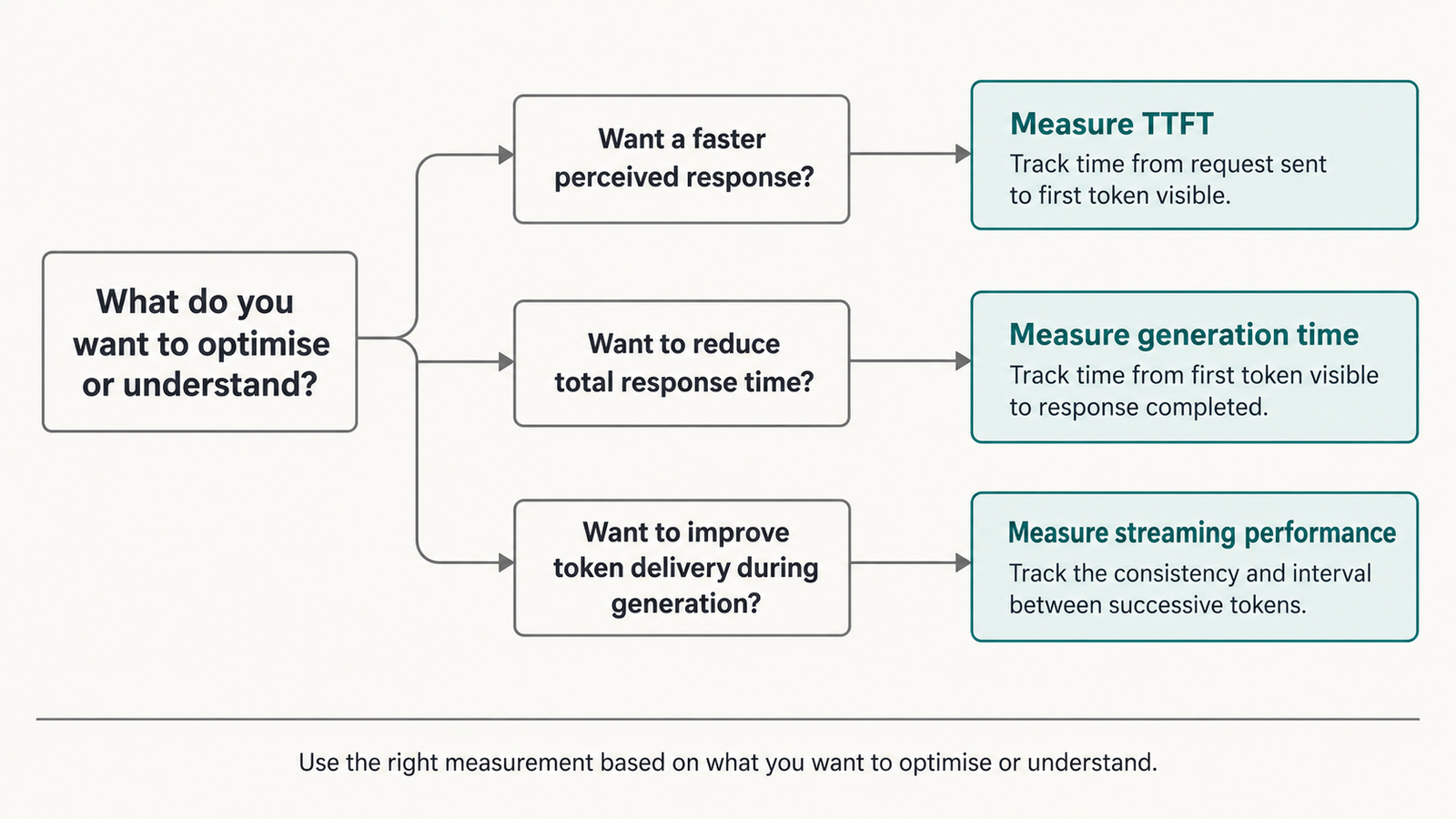
  • Time to first token (TTFT) and output speed are separate problems. A short chat reply is dominated by TTFT. A long report is dominated by output speed.
  • Agents multiply latency. Five sequential calls on a slow endpoint can take more than 100 seconds before tool time is added.
  • Published medians hide tail latency. No source examined here published p95 figures, so you have to measure them yourself.
  • Test with your own prompt lengths, region and reasoning settings before trusting any ranking, including this one.

Quick Navigation


Why LLM inference latency is hard to compare

Two published numbers for “the same model” can differ for at least six reasons that have nothing to do with the model: where the test client sits, how long the prompt is, how many requests run at once, which reasoning setting is on, how the host quantizes and batches, and which statistic is reported.

Even one careful source can disagree with itself. On Artificial Analysis’s Gemini 3.5 Flash-Lite page, the headline gives 414 tokens per second and the comparison table gives 365. Its GPT-6.1 Sol page reports a time to first answer token of 311 seconds in the headline and 327 seconds in the table. Neither page explains the gap. Different averaging windows are the likely cause, but that is an inference, not a documented fact. If a single benchmark cannot hold one number steady across its own page, rankings stitched together from several sources deserve more suspicion.

What TTFT actually measures

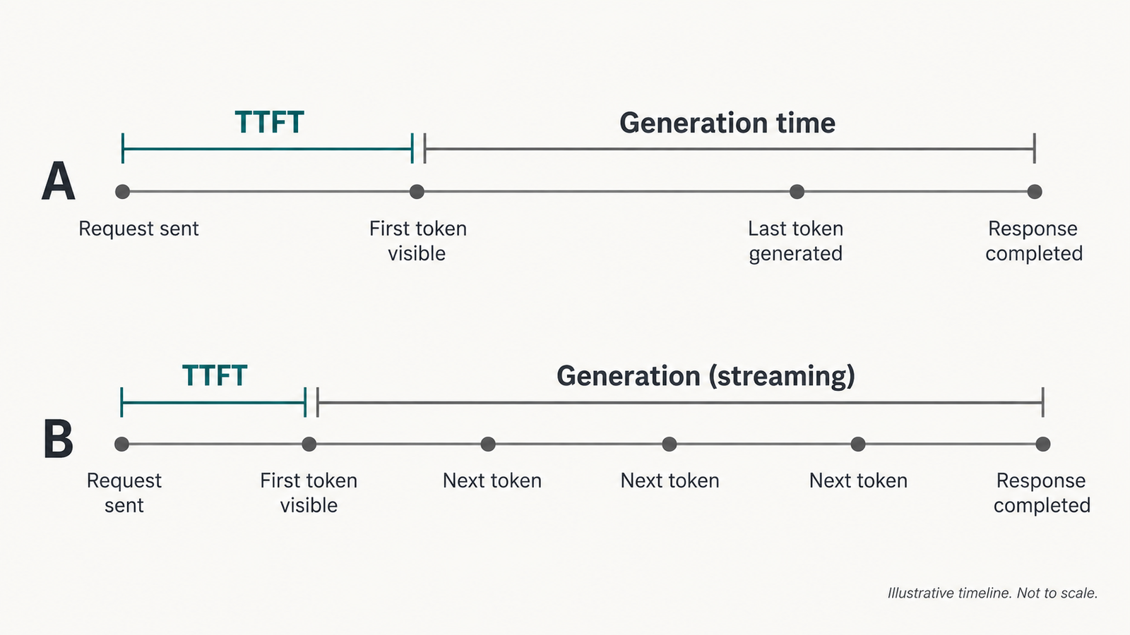
Time to first token (TTFT) is the wall-clock time between sending a request and receiving the first token of the response. Artificial Analysis’s methodology defines it that way and measures from the client.

That single number folds together several stages:

  • network time from client to provider and back
  • admission and queueing behind other customers’ requests
  • prefill, where the model processes the entire prompt before it can generate anything
  • any provider-side orchestration, such as safety checks, routing or tool-schema handling
  • for reasoning models, the thinking phase, if the measurement waits for the first answer token

Providers do not publish this breakdown, and a client-side measurement cannot separate the stages. A slow TTFT could mean a long queue, a long prompt or a distant data centre.

The reasoning point causes most of the confusion. Artificial Analysis reports two variants: TTFT to the first token of any kind, and “time to first answer token”, which includes thinking. Its per-model pages for frontier models use the second variant. That is why Claude Opus 5.5 at max effort shows roughly 600 to 1,000 seconds depending on host. The figure measures how long the model chose to think, not how fast Anthropic, Google, Azure or Amazon serve it.

TTFT versus output tokens per second

Output speed is the average rate at which tokens arrive after the first one. Artificial Analysis defines it as tokens received per second after the first token. It governs how long a full answer takes. TTFT governs how long the user stares at nothing.

The two do not move together. On Llama 3.3 70B, Google Vertex had the lowest TTFT (0.67 s) but streamed at 162 tokens/s, while SambaNova was slower to start (2.26 s) but generated faster (280 tokens/s). For a 50-token reply, Vertex wins comfortably. For a 2,000-token document, SambaNova finishes first.

The gap comes from different bottlenecks. Prefill is mostly compute-bound, processing many prompt tokens in parallel. Decode, the token-by-token generation that follows, is mostly limited by memory bandwidth, because the model’s weights stream through the chip for every token. Hardware and batching choices that help one phase can hurt the other. Large batches raise a provider’s total throughput but slow each individual stream.

LLM inference latency

LLM inference latency by model and provider

All figures are third-party measurements by Artificial Analysis, read October 11, 2026. Conditions throughout: about 10,000 input tokens, single request at a time, client in Google Cloud us-central1-a, streaming, median of the previous 72 hours. “End-to-end” is the time to receive a 500-token answer. None of this was measured by UniverseBlend.

Table 1: One model, many hosts (the controlled comparison)
ModelHostTTFT (s)Output speed (tok/s)End-to-end, 500 tokens (s)Notes
Llama 3.3 70BGoogle Vertex0.671623.76Precision not reported
Llama 3.3 70BGroq0.853282.37Custom LPU hardware
Llama 3.3 70BCoreWeave0.89787.34Not reported
Llama 3.3 70BScaleway1.48738.34Headline TTFT 1.34 s
Llama 3.3 70BTogether AI (Turbo)1.59718.65“Turbo” variant
Llama 3.3 70BNovita1.784512.83Not reported
Llama 3.3 70BAzure2.241216.38Not reported
Llama 3.3 70BSambaNova2.262804.05Headline speed 294.5
Llama 3.3 70BDeepInfra (Turbo)2.371732.53FP8
Llama 3.3 70BParasail2.57868.39FP8

Source: Artificial Analysis, Llama 3.3 70B providers. p95: not reported for any row.

Table 2: Frontier models at maximum reasoning effort
Model (API ID)HostTime to first answer token (s)Output speed (tok/s)End-to-end, 500 tokens (s)
Claude Sonnet 5.5 (claude-sonnet-5-5)Amazon475.97143479.46
Claude Sonnet 5.5Anthropic492.88142496.41
Claude Opus 5.5 (claude-opus-5-5)Google604.2595661.24
Claude Opus 5.5Anthropic704.1897667.28
GPT-6.1 Sol (gpt-6.1-sol)Azure288.6078294.99
GPT-6.1 SolOpenAI326.9456335.94

Sources: Artificial Analysis provider pages for Claude Sonnet 5.5, Claude Opus 5.5 and GPT-6.1 Sol. Effort: “max” with default fallback (Claude); “max” (GPT-6.1 Sol). These numbers mostly measure thinking time. Several Opus 5.5 rows show a time-to-first-answer longer than the 500-token total, an inconsistency the source does not explain.

Table 3: Lower-effort and lightweight endpoints (leaderboard view)
ModelHostFirst chunk (s)Output speed (tok/s)Total (s)Setting
Claude Sonnet 5.5Anthropic0.881005.86low effort
GPT-6 Luna (gpt-6-luna)OpenAI2.831256.84low effort
GPT-6.1 SolOpenAI2.804713.41low effort
Gemini 3.5 Flash-Lite (gemini-3.5-flash-lite)Google AI Studio8.9636510.33default; reasoning not reported
Qwen3.8 2.4T A95BTogether AI1.1411223.40not reported
Qwen3.8 2.4T A95BDigitalOcean0.825744.54not reported
Qwen3.8 2.4T A95BAlibaba Cloud2.993771.44not reported

Source: Artificial Analysis provider leaderboard, with Gemini from its model page. Treat this table as indicative: column values were extracted from a combined view and should be confirmed on the live page. The Qwen totals are high relative to their speed, which suggests reasoning output or longer answers. The source does not say which.

The Sonnet 5.5 rows across Tables 2 and 3 tell the main story. The same model on the same host goes from under one second to about eight minutes before answering, depending on a single API parameter.

Measurement-quality matrix
ComparisonSame model?Same harness?Same settings?Verdict
Llama 3.3 70B across hosts (Table 1)YesYesPrecision variesControlled; fair to rank, noting FP8 rows
One frontier model across clouds (Table 2)YesYesYes (max effort)Partially comparable; differences mix serving and thinking-time variance
Different frontier models (Table 2)NoYesEffort labels differ by vendorUnsuitable for a speed ranking; effort levels are not equivalent across vendors
Low-effort rows (Table 3)NoYesVariesIndicative only
Qwen across hosts (Table 3)YesYesNot reportedPartially comparable
Any of the above versus your own region and concurrencyn/aNoNoUnsuitable without retesting

How prompt length changes the first-token experience

Before a model can write its first word, it has to process every prompt token. More input means more prefill work, so TTFT generally rises with prompt length. Attention also scales worse than linearly with sequence length, which matters most at very long contexts.

In production the relationship is rarely clean. Providers split long prompts into chunks, interleave them with other customers’ work, and route long-context requests to different hardware. Artificial Analysis tests at 1,000, 10,000 and 100,000 input tokens for this reason. All the figures above use the 10,000-token workload, so they overstate TTFT for a short chat turn and understate it for a large retrieval prompt.

Caching changes the picture for repeated prefixes. Anthropic’s prompt-caching documentation says users “will generally see improved time-to-first-token for long documents” when a cached prefix is reused. Caching has no effect on output generation, and the default cache lives five minutes. The documentation gives no millisecond figure, so measure the gain on your own prompts.

Typical input sizeWhat to measure beyond the published median
Under 2,000 tokens (chat turns, classification)TTFT and first visible text from your own region; p95 under expected concurrency
2,000–30,000 tokens (RAG, documents)TTFT at three or more sizes in this range; cache-hit versus cache-miss TTFT
30,000+ tokens (codebases, long files)TTFT growth curve up to your real maximum; timeouts and error rate; whether the endpoint routes long prompts differently
Any size with a fixed system promptCached-prefix TTFT, and how quickly the cache expires under your traffic pattern

When streaming helps and when it does not

Streaming sends tokens as they are generated instead of waiting for the full response. It does not make the model faster. It changes when the user first sees something.

For a chat interface, that is often enough. Jakob Nielsen’s widely cited response-time limits, drawn from Miller (1968) and Card et al. (1991), put the edge of uninterrupted thought at about one second and the edge of sustained attention at about ten. A streamed answer that starts within a second and reads at a steady pace keeps a reader engaged, even if completion takes eight seconds.

Streaming fails in three common cases. The first is when the client needs the whole response before acting: structured JSON, a tool call or a function argument cannot be used half-written. The second is uneven cadence. Long pauses mid-stream, from server batching or client buffering in proxies and UI frameworks, can feel worse than a slightly later start. The third is reasoning models that show nothing until thinking ends, so a fast first token is meaningless if that token is hidden reasoning.

What LLM inference latency means for AI agents

This is where latency stops being a benchmark number and becomes a product problem. An agent rarely makes one call. It plans, calls a tool, reads the result and calls the model again, and every step pays TTFT and generation time in sequence.

A rough estimate per step:

T_{\text{step}} \approx \text{TTFT} + \frac{\text{output tokens}}{\text{output tokens per second}} + T_{\text{tool}}

This is an approximation. It ignores mid-stream pauses, retries and queueing spikes, and it assumes steps run one after another rather than overlapping.

The formula reproduces the source’s own totals. For Groq, 0.85 s + 500 / 328 tok/s = 2.37 s, exactly the published end-to-end figure. For DeepInfra, 2.37 + 500 / 17 = 31.8 s, against 32.5 s published.

Worked example (derived, not measured): a five-step agent, each step producing 300 output tokens and making one tool call that takes an assumed 0.8 seconds.

Endpoint (Table 1 or 2 figures)Per stepFive steps
Llama 3.3 70B on Groq0.85 + 0.91 + 0.8 = 2.56 s12.8 s
Llama 3.3 70B on Google Vertex0.67 + 1.85 + 0.8 = 3.32 s16.6 s
Llama 3.3 70B on DeepInfra (FP8)2.37 + 17.65 + 0.8 = 20.82 s104 s
Claude Sonnet 5.5, max effort, Anthropic492.88 + 2.11 + 0.8 = 495.8 sabout 41 minutes

The same five-step task is a 13-second interaction or a 41-minute background job, depending on host and settings. Neither outcome is wrong, but each implies a different product. Voice is stricter still: Stivers et al.’s 2009 PNAS study of turn-taking across 10 languages found average gaps between speakers clustering within 250 milliseconds of a cross-language mean. That points to a budget measured in hundreds of milliseconds, not seconds. That figure is a design guide drawn from human conversation, not a measured LLM threshold.

A reasonable set of engineering guidelines, labelled as such: aim for first visible text under about one second in chat, under a few hundred milliseconds of response gap in voice, and set an explicit end-to-end budget for agents, with p95 rather than median as the target.

LLM inference latency

Hosted APIs versus Llama and Qwen inference hosts

With a closed model, you can only buy latency from the vendor or the clouds that resell it. Table 2 shows that resellers can differ: GPT-6.1 Sol reached its first answer about 38 seconds sooner on Azure than on OpenAI’s own API, and streamed faster. With open weights you can also choose the serving stack, and Table 1 shows that choice matters more than anything else measured here.

That difference belongs to the host, not the model. Llama 3.3 70B is identical weights everywhere, yet output speed varies 19-fold. The causes are mostly undisclosed: accelerator type (Groq and SambaNova build their own chips), quantization (DeepInfra and Parasail are FP8), batch size and scheduling policy, and data-centre location relative to the test client. A slow host is not evidence that the model is slow, and a fast host’s numbers do not transfer to your own deployment.

Self-hosting gives you control of those variables and the responsibility for tuning them. It is also the economic question UniverseBlend examined in GPU Cloud Pricing 2026. Larger batches lower cost per token and raise per-request latency, so the cheapest configuration is rarely the most responsive one.

How to run a fair LLM inference latency test

No public benchmark matches your region, prompts and traffic. A minimal test you can run yourself:

  1. Run the client in the cloud region your users or servers actually use.
  2. Build prompts at your real input sizes, with three lengths minimum, and unique content per request so caching does not flatter results (then test cached prefixes separately).
  3. Fix output length with max_tokens and record the actual tokens returned.
  4. Set reasoning effort, temperature and tool schemas exactly as production will.
  5. Stream every request and timestamp each chunk on the client.
  6. Run at least a few hundred requests per configuration, spread across days and hours, at your expected concurrency.
  7. Report p50 and p95 for TTFT, inter-token gap and total time, plus the error and timeout rate.
import time

def measure(client, prompt, **settings):
    t0 = time.perf_counter()
    stamps = []
    for chunk in client.stream(prompt, **settings):   # provider SDK streaming call
        if chunk.text:                                  # ignore empty/keep-alive chunks
            stamps.append(time.perf_counter())
    ttft = stamps[0] - t0
    gaps = [b - a for a, b in zip(stamps, stamps[1:])]
    total = stamps[-1] - t0
    return {"ttft": ttft, "total": total,
            "max_gap": max(gaps, default=0),
            "chunks": len(stamps)}
# Run many times; report p50/p95 of each field, not the mean.

Chunks are not always single tokens, so divide counted output tokens by streaming time for a true rate. This sketch produces no results by itself, and none are reported here.

A practical provider selection framework

Pick metrics by workload before comparing providers.

CriterionMatters most whenHow to judge
TTFT at your input sizeChat, autocomplete, voicep95 from your region
Sustained output speedLong answers, reports, codeTokens per second after the first token
End-to-end completionAnything parsed as a whole (JSON, tools)p50 and p95 total time
VariabilityUser-facing productsGap between p50 and p95; largest mid-stream pause
Concurrency and rate limitsProduction trafficLatency at expected parallelism; see AI API rate limits in 2026
Tool-call overheadAgentsPer-step time multiplied by expected steps
Cost at required qualityAllCost per completed task at the reasoning setting you need

A single fastest-model ranking misleads in both directions. It can reward an endpoint that is fast because it thinks less, and penalise a model whose latency comes from a reasoning setting you would never use. Fix quality first, then compare latency among the options that meet it.

What the available evidence cannot tell us

The public data has clear gaps. It has no tail latency (medians only), one client location, mostly single-request load, and undisclosed hardware and batch sizes. Reasoning effort labels mean different things at different vendors. Frontier-model pages default to maximum effort, which few interactive products would use. Several source pages also show internal inconsistencies, so any figure here could shift by 10% or more when re-read. None of it tells you how a provider behaves during a regional incident or a demand spike, which is when latency matters most.

Conclusion

LLM inference latency becomes a product problem at a specific point: when the time a user or a downstream system must wait crosses the budget your interface was designed around. For chat that is roughly a second to first visible text. For voice it is hundreds of milliseconds. For agents it is the sum of every step, at the 95th percentile.

The evidence says the model name predicts that wait poorly. Host choice moved Llama 3.3 70B’s output speed 19-fold, and one reasoning parameter moved Claude Sonnet 5.5 from under a second to about eight minutes. Treat published rankings as a shortlist, then measure the two or three candidates yourself, with your prompts, in your region, at your load.

Frequently Asked Questions

What is a good LLM inference latency for a chatbot?

There is no universal standard. A common engineering guideline, based on Nielsen’s one-second limit for uninterrupted thought, is first visible text within about one second, with steady streaming after that. Measure p95, not just the median.

What is time to first token (TTFT)?

TTFT is the time from sending a request to receiving the first token of the response, measured at the client. It includes network time, queueing and prompt processing. For reasoning models it may also include thinking time, depending on whether the measurement waits for the first answer token.

Is TTFT or output tokens per second more important?

It depends on response length. Short replies are dominated by TTFT, and long documents by output speed. Estimate total time as TTFT plus output tokens divided by output speed for your typical response.

Why does the same open model have different latency on different hosts?

Hosts use different hardware, quantization, batching and data-centre locations. On Artificial Analysis’s October 2026 data, Llama 3.3 70B ran at 17 to 328 output tokens per second depending on host.

Why do reasoning models seem so slow in benchmarks?

Many benchmarks report time to the first answer token at the highest reasoning effort, which includes minutes of thinking. Lower effort settings respond in seconds. Compare models at the effort level you would actually use.

Does streaming reduce latency?

Streaming reduces the time until users see output, not the time to generate the full response. It helps chat, but does nothing for tool calls or structured output that must arrive complete.

Does prompt caching reduce latency?

It can reduce TTFT when a long prompt prefix repeats. Anthropic documents improved time-to-first-token for long cached documents and no effect on output generation speed. Gains depend on cache hits within the cache lifetime.

How do I benchmark LLM inference latency fairly?

Test from your production region, with your real prompt sizes and settings, streaming, at expected concurrency, over hundreds of requests across several days. Report p50 and p95 for TTFT and total time, plus errors.


Keep reading

Kimi K3.1 Pro

Kimi K3.1 Pro vs Sonnet 5.5: Same Price, Different Bill

On paper, Moonshot AI priced Kimi K3.1 Pro to the cent against Claude Sonnet 5.5: $2 per million input tokens and $10 per million output …
RAG vs fine-tuning

RAG vs Fine-Tuning: Which One You Actually Need

Take a support team that ships two prototypes on the same base model. The first searches the product documentation on every question and pastes the …
AI capex

AI Infrastructure Spending: What $145 Billion and a Sold-Out AWS Actually Buy

Published 25 October 2026 · Last verified 25 October 2026 · By the UniverseBlend editorial desk On 21 October, Meta set the latest marker for …
agentic AI

What Is Agentic AI? How AI Agents Work, What They Cost, and Where They Fail

Agentic AI describes software systems in which a language model chooses and carries out a sequence of actions to complete a task. It calls tools, …

GPU Cloud Pricing 2026: What an Hour Actually Costs

GPU cloud pricing

Published: October 2026 · Pricing last verified: October 10, 2026. Provider pricing and availability may change; check the linked source before committing to a workload.

GPU cloud pricing for the same class of NVIDIA H100 runs from $2.89 per GPU-hour on RunPod (a single H100 PCIe pod) to about $11.68 per GPU-hour on Google Cloud, where an eight-GPU a3-megagpu-8g VM lists at $93.40 an hour. Prices were checked on October 10, 2026. That is a 4x spread for one chip, but the comparison is imperfect: the cheap end is one PCIe card with 16 vCPUs, the expensive end is a full SXM node with 3,200 Gbps of networking. Newer chips sit higher still, with NVIDIA B200 at $6.69 to $14.21 per GPU-hour depending on provider and billing model.

The more useful finding is that the hourly rate is the wrong number to optimise. On a published benchmark, the most expensive chip per hour produced the cheapest tokens.

Key Takeaways
  • On-demand H100 pricing spans $2.89 to $11.68 per GPU-hour across the providers checked; H200 runs $5.29 to $10.60 and B200 $6.69 to $8.60 where an on-demand rate is published.
  • Google Cloud now lists Ironwood (TPU7x) at $12.00 per chip-hour on demand in us-central1, falling to $5.40 on a three-year commitment. TPU chip-hours are not equivalent to GPU-hours.
  • Spot and commitment discounts are larger than most provider-to-provider gaps. CoreWeave’s spot H100 node costs 60% less than its on-demand rate.
  • Using MLPerf Llama 2 70B results, an eight-GPU B200 node produced output tokens for roughly $0.15 to $0.31 per million, against $0.41 to $0.64 for an H100 node. Throughput, not rental rate, set the winner.
  • Utilisation is the cost lever buyers underestimate. At 60% productive use, a $0.48 compute cost per million tokens becomes $0.83 once modest overhead is added.
  • Price your workload in cost per million output tokens at your realistic utilisation before comparing any two quotes.

Quick Navigation


The GPU cloud pricing comparison: H100, H200, B200 and TPU7x

Every figure below comes from the provider’s own pricing page, checked October 10, 2026. Where a provider sells only eight-GPU nodes, the per-GPU figure is the node price divided by eight, shown next to the original. US regions are used unless stated. Azure and AWS on-demand rates are the exception: both companies render prices in an interactive calculator, so those two rows rely on third-party mirrors of the official price APIs and are marked as such.

ProviderAcceleratorConfigurationOn-demandReserved / committedSpot / interruptibleRegion and conditionsVerifiedSource
RunPodH100 PCIe1 GPU pod, 80 GB, 16 vCPU, 188 GB RAM$2.89/GPU-hrQuote requiredNot verifiedPer-second billing; Community vs Secure tier not distinguished in page text2026-10-10RunPod pricing
RunPodH100 SXM1 GPU pod, 20 vCPU, 125 GB RAM$3.99/GPU-hrQuote requiredNot verifiedAs above2026-10-10RunPod pricing
LambdaH100 SXM8x instance, 208 vCPU, 1,800 GiB RAM$3.99/GPU-hr ($31.92/node)Quote requiredNot offeredSelf-serve, first come; plus sales tax2026-10-10Lambda pricing
AWSH100p5.48xlarge, 8 GPU$55.04/node ($6.88/GPU), via third-party mirrorCapacity Block $47.757/node ($5.97/GPU)Varies by zoneus-east-1; Capacity Blocks prepaid, price updates next January 20272026-10-10AWS Capacity Blocks
CoreWeaveH100HGX node, 8 GPU, 128 vCPU, 2 TB RAM$49.24/node ($6.16/GPU)Up to 60% off, quote required$19.71/node ($2.46/GPU)North America; egress free2026-10-10CoreWeave pricing
Google CloudH100a3-highgpu-8g, 8 GPU$88.49/node ($11.06/GPU)1-yr $61.38; 3-yr $38.86$50.32/nodeus-central1; spot price variable2026-10-10Google accelerator pricing
Google CloudH100a3-megagpu-8g, 8 GPU$93.40/node ($11.68/GPU)1-yr $64.21; 3-yr $40.65$53.10/nodeus-central12026-10-10Google accelerator pricing
AzureH100ND96isr H100 v5, 8 GPU$98.32/node ($12.29/GPU), via third-party mirrorNot verifiedNot verifiedEast US; official page renders client-side2026-10-10Azure VM pricing
RunPodH2001 GPU pod, 141 GB, 24 vCPU$5.29/GPU-hrQuote requiredNot verifiedInstant cluster rate $4.31/GPU-hr2026-10-10RunPod pricing
CoreWeaveH200HGX node, 8 GPU$50.44/node ($6.31/GPU)Quote required$20.93/nodeNorth America2026-10-10CoreWeave pricing
AWSH200p5e.48xlarge, 8 GPUNot verifiedCapacity Block $54.924/node ($6.87/GPU)Not verifiedUS East (Ohio), US West2026-10-10AWS Capacity Blocks
Google CloudH200a3-ultragpu-8g, 8 GPU$84.81/node ($10.60/GPU)1-yr $58.47; 3-yr $37.21$50.83/nodeus-central12026-10-10Google accelerator pricing
LambdaB200 SXM68x instance, 180 GB/GPU$6.69/GPU-hr ($53.52/node)1-Click Cluster, 2 wk–1 yr: $8.87–$9.86/GPU-hrNot offeredSelf-serve2026-10-10Lambda pricing
RunPodB2001 GPU pod, 180 GB, 28 vCPU$7.99/GPU-hrQuote requiredNot verifiedPer-second billing2026-10-10RunPod pricing
CoreWeaveB200HGX node, 8 GPU$68.80/node ($8.60/GPU)Quote required$34.11/node ($4.26/GPU)North America2026-10-10CoreWeave pricing
Google CloudB200a4-highgpu-8g, 8 GPUNot offered on demand1-yr $88.93; 3-yr $56.71; DWS Flex-start $64.44$39.63/nodeus-central12026-10-10Google accelerator pricing
AWSB200p6-b200.48xlarge, 8 GPUNot verifiedCapacity Block $113.666/node ($14.21/GPU)Not verifiedus-east-1, us-east-2, us-west-22026-10-10AWS Capacity Blocks
Google CloudIronwood (TPU7x)Per chip$12.00/chip-hr1-yr $8.40; 3-yr $5.40Variableus-central1; London $13.202026-10-10Cloud TPU pricing

Not verified as publicly available: H200 and B200 on Lambda’s self-serve instance list, B200 on Azure, and any TPU outside Google Cloud. Azure H200 and B200 pricing could not be confirmed from an official page in this pass.

Two things stand out. Google prices the same H100 at nearly four times RunPod’s PCIe rate, but the Google VM bundles 208 vCPUs, 1.87 TB of RAM, 6 TB of local SSD and multi-node networking. And Google sells B200 only through commitments, spot or its Dynamic Workload Scheduler, so there is no plain on-demand rate to compare.

What the hourly GPU cloud price does not tell you

An hourly rate prices access to hardware. It says nothing about how much of that hardware your model will use, or what else the bill will carry.

  • Memory decides how many GPUs you rent. A 70-billion-parameter model in FP8 needs roughly 70 GB for weights alone, before the KV cache that holds each conversation’s context. That fits on one 141 GB H200 with room for batching, but is tight on an 80 GB H100, which pushes many teams to two or more cards. The H200’s higher hourly rate can therefore buy a smaller bill.
  • Bandwidth sets decode speed. Generating each output token means streaming the model’s weights through the GPU’s memory. AWS describes the B200 instances as offering 1.6x the GPU memory bandwidth of P5en, which matters more for token output than headline FLOPS.
  • The node is not just GPUs. CoreWeave’s H100 node includes 128 vCPUs, 2 TB of RAM and 61 TB of local NVMe; a RunPod H100 SXM pod includes 20 vCPUs and 125 GB. Data loading, tokenisation and preprocessing all run on that host side.
  • Egress and storage vary sharply. CoreWeave and Lambda advertise no egress fees, while AWS bills data transfer out to the internet beyond a free 100 GB a month. Storage left attached to stopped instances keeps billing: RunPod charges $0.20 per GB-month for idle volume disks, double the running rate.
  • Idle time is the largest hidden cost. Google bills a one-minute minimum, then per second, and charges a VM that is idle but RUNNING at full rate. A cluster that waits overnight for the next job costs exactly as much as one serving traffic. As UniverseBlend’s 2026 AI accelerator comparison put it, a rack at 30% use costs about three times as much per token as the same rack at 90%.

On-demand, reserved and spot GPU cloud pricing

  1. On-demand suits work measured in hours or days: experiments, evaluation runs, short fine-tunes. You pay the highest rate for the right to stop.
  2. Reservations and commitments pay off when the GPUs would otherwise run continuously. The published discounts are not alike, though. Google’s 1-year commitment on an a3-highgpu-8g cuts the hourly rate from $88.49 to $61.38, and the 3-year rate to $38.86; Google also notes that reserved resources bill whether or not they are running. AWS Capacity Blocks work differently again: you prepay a fixed window up front, at a rate AWS revises on a published schedule. CoreWeave advertises “up to 60%” off for committed use but publishes no rate, so that discount is a ceiling, not a price.
  3. Spot and preemptible capacity is cheapest on paper and riskiest in practice. CoreWeave lists its spot H100 node at $19.71 an hour, against $49.24 on demand. Google says spot prices can change up to once a day and VMs can be preempted at any time.

Interruption has a measurable cost. Suppose a training job checkpoints every hour and a preemption loses, on average, 30 minutes of work plus 15 minutes to restart. If that happens once every 10 hours, the job does 10 hours of useful work in about 10.75 billed hours. At CoreWeave’s spot rate, that is $19.71 × 10.75 / 10 = $21.19 per useful node-hour, still 57% below on demand. Spot stops paying when preemptions become frequent enough that restart time dominates, or when a deadline cannot absorb the delay. These interruption figures are illustrative assumptions, not measured provider rates.

One caution when comparing discounts across clouds: Google’s committed price, AWS’s prepaid block and CoreWeave’s quoted reservation buy different things, with different cancellation terms and different guarantees of capacity in a specific zone. Compare the effective hourly rate over the full term you would actually commit to.

From GPU cloud pricing to cost per million tokens

The number that matters for inference is what a million output tokens cost. Converting an hourly rate needs only one more figure, sustained output throughput:

\text{Cost per million output tokens} = \frac{\text{hourly compute cost} \times 1{,}000{,}000}{\text{output tokens per second} \times 3{,}600}

As a mathematical illustration only: an instance costing $2.00 an hour that produces 100 output tokens per second costs $2.00 × 1,000,000 / 360,000 = $5.56 per million output tokens.

GPU cloud pricing
The throughput evidence

No provider publishes token throughput for its own instances, so this analysis uses MLPerf Inference, the industry benchmark run under audited rules by MLCommons. The workload is Llama 2 70B in the Closed division, Server scenario, which imposes latency limits closer to live serving than the batch-oriented Offline scenario. Throughput is aggregate output tokens per second across all concurrent requests on an eight-GPU system, not the speed any single user sees.

  • B200: 102,398 tokens/s on an 8x B200 SXM system (CoreWeave), MLPerf Inference v6.1, reported by NVIDIA, page dated October 2026. Blackwell submissions on this benchmark use FP4 weights.
  • H200: 29,228 tokens/s on 8x H200 without Triton, MLPerf Inference v4.1, August 2024, TensorRT-LLM with FP8.
  • H100: about 21,500 tokens/s for 8x H100. This is derived, not measured here: NVIDIA’s v4.1 post gives 10,756 tokens/s for one B200 and states that equals 4x the H100’s per-GPU result. 10,756 / 4 × 8 ≈ 21,512.

These figures do not compare like with like. The B200 result is two years newer, uses FP4 rather than FP8, and benefits from two years of software tuning that the Hopper numbers do not capture. Hopper’s cost per token today is probably somewhat lower than shown. The gap is still too wide for that to reverse the ranking.

Results
Accelerator / providerHourly cost (8-GPU node)Output throughputCompute cost per 1M output tokensAssumptions and source
B200 / CoreWeave spot$34.11102,398 tok/s$0.09MLPerf v6.1 Server; spot, interruptible
B200 / Google A4 spot$39.63102,398 tok/s$0.11As above; Google spot
B200 / Lambda$53.52102,398 tok/s$0.15$6.69 × 8; on demand
B200 / CoreWeave$68.80102,398 tok/s$0.19On demand
B200 / AWS Capacity Block$113.67102,398 tok/s$0.31Prepaid block
H200 / CoreWeave spot$20.9329,228 tok/s$0.20MLPerf v4.1 Server, FP8; spot
H200 / RunPod cluster$34.4829,228 tok/s$0.33$4.31 × 8
H200 / CoreWeave$50.4429,228 tok/s$0.48On demand
H200 / AWS Capacity Block$54.9229,228 tok/s$0.52p5e; prepaid
H200 / Google A3 Ultra$84.8129,228 tok/s$0.81On demand
H100 / Lambda$31.92~21,512 tok/s (derived)$0.41$3.99 × 8
H100 / AWS Capacity Block$47.76~21,512 tok/s (derived)$0.62Prepaid block
H100 / CoreWeave$49.24~21,512 tok/s (derived)$0.64On demand

The B200 node at CoreWeave costs 40% more per hour than the H100 node, yet produces each token for less than a third of the price. That is the whole argument for pricing in tokens: a 4.8x throughput gap overwhelms a 1.4x price gap. It also explains why serving workloads are migrating to newer silicon faster than training, a split UniverseBlend examined in inference chips versus training chips.

These are compute-only estimates. They assume the GPUs run at MLPerf throughput every second of every hour, with prompts and outputs shaped like the benchmark’s OpenOrca dataset (sequences capped at 1,024 tokens). Your prompts, context lengths and latency targets will move the result, and none of these figures include storage, networking, redundancy or engineering time.

Against a hosted API

Together AI lists Llama 3.3 70B at $1.04 per million tokens, input and output alike. That is a newer model than the Llama 2 70B benchmark, so treat the comparison as rough. Even so, the API costs roughly two to eleven times the compute-only estimates above, and buys something real for the difference: no idle hours, no minimum commitment, and someone else handling scaling and failures. Self-hosting wins only if you can keep the hardware busy. A node at 20% utilisation multiplies every figure in the table by five.

A reusable GPU cost calculator

Five inputs are enough to estimate your own cost per million output tokens: hourly instance price, number of instances, measured output tokens per second, productive utilisation, and non-GPU hourly overhead.

  1. Effective hourly cost = instance hourly cost × number of instances + additional hourly overhead
  2. Effective token throughput = measured output tokens per second × 3,600 × utilisation fraction
  3. Cost per million output tokens = effective hourly cost × 1,000,000 / effective token throughput

Utilisation here means the share of paid time spent generating tokens at the measured rate. If your throughput figure already came from a production trace that includes idle gaps, set utilisation to 100% so you do not count the idle time twice.

Worked example. One CoreWeave H200 node at $50.44 an hour, an assumed $2.00 an hour for storage, monitoring and a load balancer, MLPerf throughput of 29,228 tokens per second, and 60% productive utilisation:

  • Effective hourly cost: $50.44 × 1 + $2.00 = $52.44
  • Effective throughput: 29,228 × 3,600 × 0.60 = 63,132,480 tokens per hour
  • Cost: $52.44 × 1,000,000 / 63,132,480 = $0.83 per million output tokens

That is 73% above the $0.48 compute-only figure, from utilisation and a small overhead alone. Real production budgets also carry engineering time, redundancy, retries and orchestration. Treat this as a floor, not a forecast. For a fuller total-cost model that weighs hosted and owned capacity, UniverseBlend’s analysis of AMD’s hybrid AI TCO calculator works through the assumptions behind those vendor tools.

Which provider fits which workload

The published prices support conditional advice rather than a single winner.

  • Short experiments and development: single-GPU, per-second pods such as RunPod’s are the cheapest way to get an H100 for an afternoon. Check the host vCPU and RAM before loading a large dataset.
  • Fine-tuning and training: multi-GPU jobs need fast GPU-to-GPU links. Full SXM nodes from Lambda, CoreWeave, AWS or Google are the safer choice; a set of separate single-GPU pods is not a substitute.
  • Sustained inference: price in tokens. On the evidence above, B200 nodes produced the lowest compute cost per token, and Lambda’s on-demand B200 was the cheapest non-interruptible option checked.
  • High-throughput batch generation: spot capacity fits, provided jobs checkpoint. CoreWeave’s and Google’s spot B200 rates gave the lowest token costs in this analysis.
  • Bursty workloads: a hosted API or a serverless endpoint usually beats a reserved node, because you stop paying for the troughs.
  • Production that cannot tolerate interruption: on-demand or committed capacity only. Google B200 requires a commitment or scheduler-based capacity; AWS publishes prepaid Capacity Blocks.
  • Teams needing a specific generation: Google is the only provider here offering TPU7x. AWS lists B200 through Capacity Blocks in nine regions. Lambda’s self-serve list shows B200 and H100 but not H200.

The evidence cannot settle reliability, real capacity in a given week, or support quality. Those need a trial and a written commitment.

How to check a GPU cloud quote before you sign

  • Exact instance type and accelerator count, including SXM versus PCIe
  • Region and zone, with written confirmation that capacity exists there
  • Billing unit and minimum: per second, per minute, per hour or prepaid block
  • Included vCPUs, host RAM, local NVMe and attached storage
  • Network egress and inter-region transfer charges
  • Commitment length, cancellation terms and whether unused hours are billed
  • Preemption policy and notice period for spot capacity
  • Your own measured throughput on your model, not a vendor benchmark
  • Realistic utilisation, including nights and weekends
  • Monitoring, orchestration and support costs

Conclusion

GPU cloud pricing is published more openly than at any point in the past three years. Most providers here publish usable rates on static pages; AWS and Azure still keep on-demand rates inside calculators, and Google now lists Ironwood. The problem has shifted from finding a price to interpreting one.

The numbers point one way. The cheapest hour checked was a $2.89 H100 PCIe pod; the cheapest tokens came from an eight-GPU B200 node costing more than $50 an hour. Buyers who compare rental rates will choose the wrong hardware. Measure throughput on your own model, assume honest utilisation, and compare quotes in dollars per million output tokens.

Maintenance note: review this table monthly, and whenever a provider launches a new accelerator, changes a price, or revises billing terms. Record the real verification date for each changed row.

Frequently Asked Questions

How much does it cost to rent an H100 GPU per hour in 2026?

As of October 10, 2026, on-demand H100 prices ran from $2.89 per GPU-hour for a single PCIe pod on RunPod to $11.68 per GPU-hour on a Google Cloud a3-megagpu-8g VM. Full eight-GPU SXM nodes from Lambda and CoreWeave list at $3.99 and $6.16 per GPU-hour.

Is an H200 more expensive than an H100?

Usually, but not everywhere. RunPod charges 33% more ($5.29 versus $3.99 per GPU-hour) and CoreWeave about 2% more per node, while Google’s H200 a3-ultragpu-8g VM ($84.81) is cheaper than its H100 a3-highgpu-8g ($88.49). With 141 GB of memory and higher measured throughput, H200 often costs less per token.

How much does an NVIDIA B200 cost per hour?

Public rates ranged from $6.69 per GPU-hour on Lambda to $14.21 per GPU-hour on an AWS Capacity Block. CoreWeave lists $8.60 on demand and $4.26 on spot. Google offers B200 only through commitments, spot or its Dynamic Workload Scheduler.

Does Google Cloud publish TPU v7 pricing?

Yes. Google’s Cloud TPU pricing page lists Ironwood (TPU7x) at $12.00 per chip-hour on demand in us-central1, $8.40 on a 1-year commitment and $5.40 on a 3-year commitment. Prices are per chip, not per VM, and are not directly comparable with GPU-hours.

Is spot GPU pricing worth the interruption risk?

For checkpointed training and batch jobs, usually yes: CoreWeave’s spot H100 node costs 60% less than on demand, leaving room to absorb lost work. For latency-sensitive production serving, no, because a preemption becomes an outage.

Is renting a GPU cheaper than using an AI API?

Only at high utilisation. Compute-only costs on rented 70B-class serving ranged from about $0.09 to $0.81 per million output tokens at full benchmark load, against $1.04 for Llama 3.3 70B on Together AI’s API. Below roughly 20% to 60% utilisation, depending on hardware and rate, the API is often cheaper.

How do I calculate GPU inference cost per million tokens?

Multiply the hourly cost by 1,000,000, then divide by output tokens per second × 3,600 × your utilisation fraction. Use throughput measured on your own model and prompt lengths.

What additional costs should I include in a GPU cloud budget?

Storage, data egress, idle time, host CPU and memory, monitoring, orchestration, redundancy and engineering time. Idle time is usually the largest, because most providers bill a running instance whether or not it does useful work.


Keep reading

Kimi K3.1 Pro

Kimi K3.1 Pro vs Sonnet 5.5: Same Price, Different Bill

On paper, Moonshot AI priced Kimi K3.1 Pro to the cent against Claude Sonnet 5.5: $2 per million input tokens and $10 per million output …
RAG vs fine-tuning

RAG vs Fine-Tuning: Which One You Actually Need

Take a support team that ships two prototypes on the same base model. The first searches the product documentation on every question and pastes the …
AI capex

AI Infrastructure Spending: What $145 Billion and a Sold-Out AWS Actually Buy
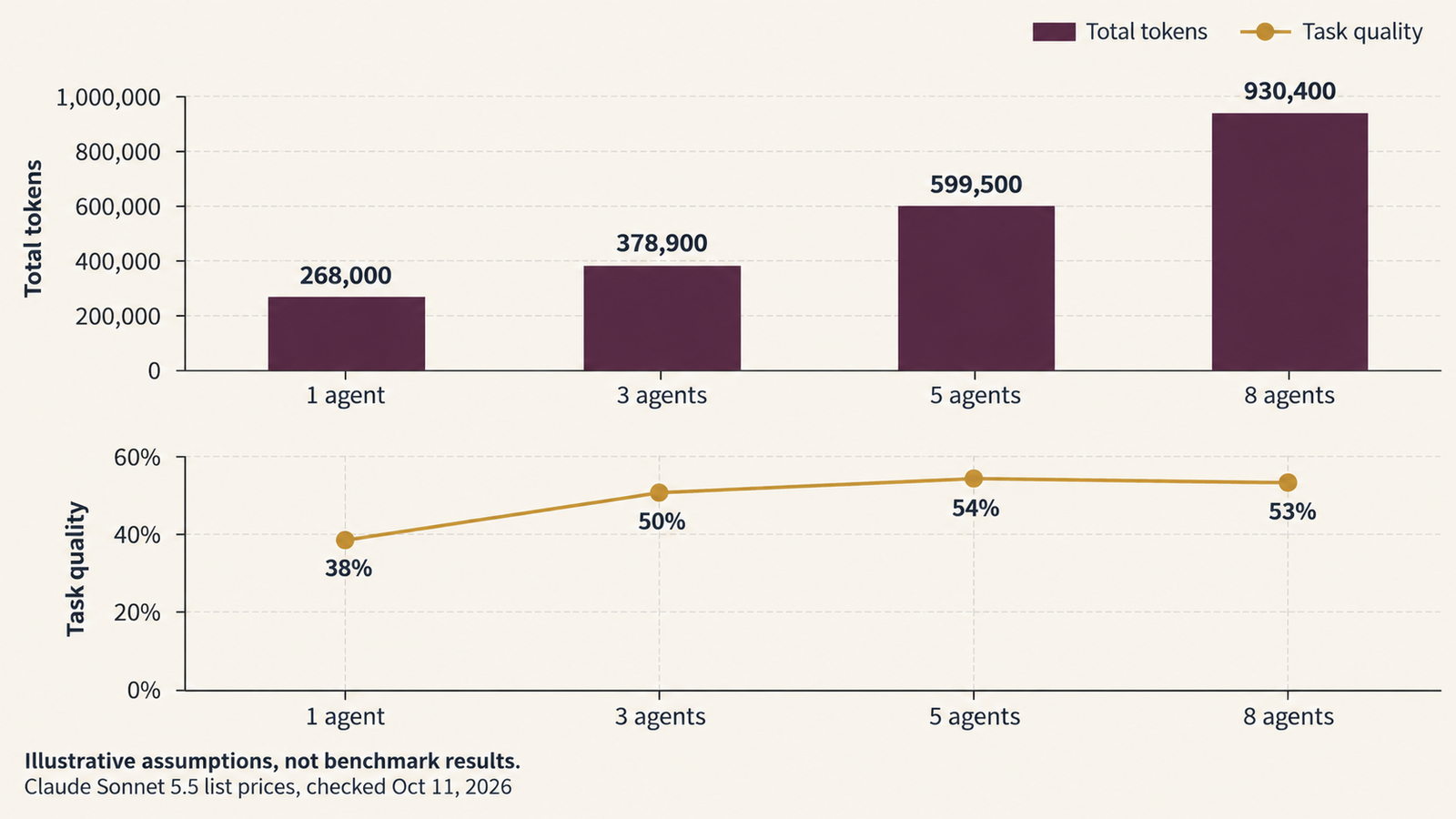
Published 25 October 2026 · Last verified 25 October 2026 · By the UniverseBlend editorial desk On 21 October, Meta set the latest marker for …
agentic AI

What Is Agentic AI? How AI Agents Work, What They Cost, and Where They Fail

Agentic AI describes software systems in which a language model chooses and carries out a sequence of actions to complete a task. It calls tools, …

The $60B AI Chip Financing and Its Residual-Value Problem

AI chip financing

A lender writing a $42 billion senior secured cheque asks two questions. Can the borrower pay? And if it cannot, what is the security worth?

For most asset-backed lending the second question is the easy one. Property has comparable sales. Aircraft have a global resale market and published values. Vehicles have auction data going back decades. The collateral has a price history that exists independently of the borrower.

AI accelerators do not have that yet. They have a list price, an accounting schedule and a thin secondary market whose depth has never been tested at scale in a downturn. The debt being written against them is real and large; the recovery assumption underneath it is a judgement.

That gap is the subject here. The $60 billion package syndicating this week is a bet on Anthropic’s business and, simultaneously, a bet on what a 2027-generation TPU is worth in 2030.

Key takeaways
  • The Financial Times reported on October 6 that Bank of America, Citigroup and Morgan Stanley began syndicating a $60 billion debt package funding Anthropic’s lease of Google-designed chips: roughly $42 billion of senior secured debt backstopped by Broadcom and $18 billion of junior debt, with Blackstone committing about $9 billion of the latter.
  • Some syndicated coverage published the same figures inflated tenfold. The correct numbers are $42bn, $18bn and $9bn.
  • This $60 billion is separate from Anthropic’s reported $518 billion of total compute commitments. The financing funds part of the commitments; it is not the same number.
  • Book value, market value and recovery value are three different things, and only the third matters in a workout. The gap between them widens when a technology generation turns.
  • The aircraft analogy is useful for structure and misleading on liquidity. Aircraft have thousands of potential operators worldwide; frontier accelerators have a buyer pool measured in dozens.
  • The distinctive risk is correlation: the conditions that stress the borrower are the same conditions that soften demand for the collateral. Borrower risk and collateral value can deteriorate together.
  • Credit markets have started pricing this. PGIM anchored a $500 million CLO in late September containing a first-of-its-kind 15% cap on AI-related collateral.

Quick Navigation


The $60 Billion Transaction, Stripped to Mechanics

What the Financial Times reported, and what subsequent coverage corroborates:

ElementDetail
ArrangersBank of America, Citigroup, Morgan Stanley
Total package$60 billion
Senior tranche~$42 billion, secured, backstopped by Broadcom
Junior tranche~$18 billion, no Broadcom guarantee
Junior anchorBlackstone, committing ~$9 billion and syndicating the rest
PurposeFunding Anthropic’s chip orders through 2027
Payment startLease payments commence after chip delivery
StatusSyndication letters out; books not closed

The economic shape is a leasing structure rather than a purchase. A financing vehicle funds the hardware, Anthropic leases it, and the lease payments service the debt. Anthropic does not own the chips, which is precisely why the hardware can serve as security for the senior lenders.

Two features deserve attention before anything else.

  1. The Broadcom backstop is doing enormous work. The senior tranche is supported by Broadcom’s investment-grade credit, widely reported as A−. That is what makes $42 billion placeable with institutional lenders at a manageable cost. Without it, the senior tranche would be priced against the credit of a company that reported a $42 billion net loss in 2025, most of it non-cash, with revenue of $4.59 billion.
  2. The junior tranche is the honest price signal. The $18 billion with no guarantee sits directly against Anthropic’s credit and the hardware. Blackstone taking half of it is a meaningful commitment; the terms on which the rest places will tell you more about market appetite than any amount of commentary.

Timing matters too. Payments begin after delivery in 2027. The debt is being raised now against cash flows that start later, which means the underwriting rests on a forecast of Anthropic’s 2027–2032 revenue and on a residual-value assumption for hardware that does not yet exist in the data centre.

What AI Chip Financing Actually Means

AI chip financing is the use of debt to fund the acquisition or lease of AI accelerators, where the hardware and the contracted payments it generates serve as the basis for repayment. It is equipment finance applied to silicon that depreciates faster than almost anything else lenders have taken as security.

The arrangements differ more than the headlines suggest:

StructureWho owns the hardwareWho carries the residual risk
Outright purchaseThe buyerThe buyer
Operating leaseThe lessorThe lessor
Finance leaseEffectively the lesseeThe lessee
Asset-backed debtA financing vehicleLenders, through the security package
Vendor financingVariesThe vendor, partly
Credit guaranteeUnchangedThe guarantor, on default

The Anthropic structure combines several of these at once: a lease to the user, asset-backed debt to fund it, a guarantee from the chip supplier on the senior piece, and a separate convertible facility from that same supplier.

Senior and junior, without oversimplifying
  • Senior secured debt holds a first claim on pledged collateral and sits at the top of the repayment waterfall. In this structure it also carries Broadcom’s support, which means a senior lender has two sources of recovery: the guarantee and the security.
  • Junior debt ranks behind. It absorbs losses first, prices wider to compensate, and here it carries no guarantee at all.

The simplification worth flagging: priority is set by intercreditor agreements and the specific security package, not by the labels. What assets are actually pledged, whether the pledge is over the hardware or over the equity of the vehicle that owns it, how enforcement works across jurisdictions, and what conditions govern the guarantee all matter more than the words “senior” and “junior.” Those documents are not public.

For a lender, this means the senior position is substantially a Broadcom credit exposure with hardware as backup, while the junior position is a direct bet on Anthropic and on what the chips fetch. Those are very different risks wearing the same deal name.

Three Different Values, Only One of Which Matters in a Workout

Every asset has three values, and conflating them is how collateral analysis goes wrong.

ValueWhat it isWho uses it
Book valueOriginal cost less accumulated depreciation, per the schedule chosenAccountants, auditors, the income statement
Market valueWhat a willing buyer pays a willing seller in an orderly marketAsset managers, insurers, secondary traders
Recovery valueWhat a lender actually realises after default, enforcement, delay, remarketing and costsCredit analysts, workout desks

Recovery value is the only one that protects a lender, and it is always the lowest of the three. The discount between market and recovery reflects time, transaction costs, the circumstances of a forced sale, and whether a buyer exists when you need one.

For AI accelerators, several factors widen that discount specifically:

  • Integration. A rack of accelerators is not a commodity unit. It needs compatible networking, power delivery, cooling and a software stack. Recovering value may mean selling a system, not a chip.
  • Location. The hardware sits in a data centre with its own lease, power contract and operator. Physical recovery is not simply a repossession.
  • Operating cost. Unlike an aircraft in storage, idle accelerators in a facility still consume rent and, if kept warm, power.
  • Timing. Enforcement takes months. A technology generation can turn in twelve.

Accounting Depreciation Is Not Economic Depreciation

Accounting depreciation allocates cost across a chosen useful life. It is a smooth line, usually straight, and it is an estimate made by management.

Economic depreciation is what the asset is actually worth over time, and it is not smooth at all. It is flat while the hardware remains the current generation, then steps down sharply when a materially better part ships, then flattens again at whatever floor the installed base supports.

The mismatch matters because book value follows the first curve and recovery value follows the second. A chip carried at 60% of cost on a six-year schedule may be worth considerably less in a market where the new generation delivers substantially more performance per watt.

We argued in our analysis of AI accelerator depreciation that these schedules are among the least audited assumptions in AI infrastructure economics, and that memory capacity rather than compute is often what ends an accelerator’s competitive life. That was an accounting and modelling point. The $60 billion package turns it into a credit question, because a residual-value assumption that was previously internal to a company’s financial statements is now embedded in the security package for institutional debt.

The key distinction is this: book value is an assertion, market value is an observation, and recovery value is an outcome. Only the first is visible in advance.

Where the Aircraft Analogy Works, and Where It Breaks

Bankers reach for aircraft finance when explaining these structures, and the comparison deserves better than dismissal. Aviation leasing is a mature, multi-decade, trillion-dollar market that solved several problems this one now faces.

Where the analogy genuinely holds:

  • A high-value physical asset with a long nominal life
  • Lease structures separating ownership from operation
  • Asset-backed debt with residual-value assumptions baked into pricing
  • Specialist lessors who understand the equipment better than the lenders do
  • Established enforcement mechanics for repossession
  • Cash flows contracted in advance from creditworthy operators

That is a real set of similarities, and it explains why the structure was reachable at all.

Where it breaks, and the breaks are substantial:

Commercial aircraftAI accelerators
Potential buyersHundreds of airlines and lessors worldwideDozens of hyperscalers, labs and specialist clouds
Useful life20–30 yearsCompetitive life measured in years
Obsolescence driverFuel efficiency, gradualNew generation, stepwise
Secondary marketDeep, priced, with published appraisalsThin, opaque, largely untested in stress
PortabilityFly it to the new operatorDecommission, ship, reinstall, reintegrate
Software dependenceMinimalSubstantial — ecosystem compatibility matters
Operating economicsOlder aircraft remain viable on secondary routesOlder accelerators compete directly on performance per watt

The buyer-pool difference is the one that does most of the damage to the analogy. When a regional carrier fails, its narrowbodies find homes because thousands of operators fly that type and demand for air travel is not correlated with that carrier’s solvency. When a large AI lab’s economics deteriorate, the set of organisations able to absorb tens of thousands of accelerators is small, and they are mostly reading the same market signals.

There is also a specificity problem. The TPUs in this transaction are designed for a particular architecture and ecosystem. The resale question is not “what is a GPU worth” but “who else runs this hardware, at scale, with the networking and software to use it.” That is a narrower question than it sounds.

The Correlated-Collateral Problem

Good collateral is uncorrelated with the borrower. That is the whole point of taking security: when the borrower fails for borrower-specific reasons, the asset retains value because its market has other participants and other drivers.

AI accelerators may not offer that separation.

The mechanism, stated as analysis rather than prediction:

AI demand weakens → borrower revenue and cash flow come under pressure → default risk rises → demand for AI accelerators weakens across the sector → secondary-market prices fall → recovery value declines.

Every arrow in that chain is driven by the same underlying variable. The thing that would cause Anthropic to struggle — a slowdown in enterprise AI spending, a compression in model pricing, a capability plateau — is the same thing that would thin the buyer pool for its hardware.

AI chip financing

Compare that with the aviation case. An airline fails because of its route network, its balance sheet or a labour dispute; aircraft values barely move, because demand for air travel is intact and other operators are buying. The collateral is insulated from the borrower’s problem.

Here the insulation is weaker. The important risk is not borrower credit alone, and not residual value alone. It is the interaction between them.

Two qualifications keep this honest.

  1. This is a risk characteristic, not a prediction of crisis. Correlated collateral is common in structured finance — commercial mortgages in a single metro, shipping in one trade lane — and markets price it rather than refuse it. The question is whether it is being priced.
  2. The correlation is imperfect. A borrower-specific failure, as opposed to a sector downturn, would leave hardware demand intact and recovery would look much better. Anthropic losing share to a competitor is a different scenario from AI spending flattening industry-wide, and only the second produces the full correlation effect.

The practical consequence for a credit analyst: stress-testing this exposure requires modelling borrower default and collateral value as joint outcomes, not as independent variables multiplied together. Treating them as independent will understate loss severity in exactly the scenario that matters.

Broadcom Occupies Three Seats at the Table

State this plainly, because it is unusual and it is disclosed rather than hidden.

RoleWhat it means
SupplierBroadcom produces the custom accelerators Anthropic is leasing
GuarantorIts investment-grade credit backstops the ~$42bn senior tranche
LenderPer Broadcom’s quarterly report and a term sheet shown to investors, Anthropic could issue up to $42 billion of convertible notes to Broadcom to cover lease payments

The economic exposures run in different directions and are worth separating.

As supplier, Broadcom books revenue on hardware it sells into the structure. As guarantor, it takes contingent credit exposure to Anthropic’s performance. As convertible lender, it takes direct credit exposure that could convert into equity. Reporting indicates Anthropic is on track to become Broadcom’s largest custom-silicon customer.

What that combination produces, as analysis: Broadcom’s revenue from this customer is partly financed by Broadcom’s own credit. If the customer performs, the company captures product margin plus the upside on a convertible position. If the customer struggles, it absorbs losses as guarantor and as lender simultaneously, on top of losing the revenue.

This is not a scandal and it is not novel in kind. Vendor financing is as old as capital equipment, and Anthropic’s own prospectus reportedly flags potential conflicts of interest, warning that Broadcom’s decisions on pricing and hardware could affect Anthropic’s ability to procure enough compute. Both parties have disclosed the arrangement.

What it does mean for a senior lender is specific: the guarantee that makes the paper investment-grade comes from a party whose own exposure to the same borrower is large and multi-layered. The guarantee is not independent of the risk it covers. That is a correlation of a different kind, sitting on top of the collateral correlation already described.

What the Credit Market Is Signalling

The interesting response is not commentary. It is documentation.

On September 29, Bloomberg reported that PGIM anchored a $500 million CLO issued by Allstate containing a first-of-its-kind provision capping AI-related collateral at 15% of the pool. PGIM’s co-head of securitized products indicated the firm is exploring similar structures with other managers and is building a framework to assess loans by their AI-sector linkage.

That is a structural response rather than a view. A manager that thought AI credit was simply attractive would buy more of it; a manager that thought it was simply bad would avoid it. Capping it means treating the exposure as acceptable but correlated.

Two further data points, both attributed carefully. Bank of America strategists have been reported as estimating that CLO exposure to chips and data centres could approach $100 billion; I could not locate the underlying note, so treat it as a strategist estimate. Separately, JPMorgan has put up to $150 billion of CLO-held leveraged loans in sectors facing meaningful AI-disruption risk — a different measure of a different thing, and not additive with the first.

For the market, this means AI infrastructure has moved from an equity story to a credit story. The relevant question changes from how much upside a successful build-out produces to how losses are distributed if it disappoints — and that question is answered by security packages and recovery assumptions, not by growth forecasts.

The Case for the Collateral Holding Its Value

The bearish reading is easy to write and may well be wrong. Several arguments point the other way, and lenders taking this paper are not naive.

  • Scarcity is the strongest one. Advanced accelerators have been supply-constrained for three years. Memory is the binding input and it is contracted years ahead — Micron said in September that it had committed the vast majority of its calendar 2027 HBM supply at significantly higher prices, which we covered in our analysis of HBM pricing for 2027. Hardware that is hard to obtain new holds its value used.
  • Inference workloads extend useful life. The frontier-training use case has the shortest competitive half-life. Serving established models is less demanding, and older accelerators often remain economic for inference long after they stop being the right choice for training. That gives the installed base a floor that pure training economics would not.
  • Utilisation, not vintage, determines productivity. A fully utilised previous-generation fleet can produce better economics than an underutilised current-generation one, which is the argument we made in our analysis of accelerator utilisation. A buyer with demand to fill will take older hardware at the right price.
  • Demand is broadening. Sovereign programmes, enterprises and specialist clouds have entered the market. The buyer pool is thin compared with aviation, but it is thicker than it was two years ago.
  • Power is becoming the constraint. If electrical capacity rather than silicon limits deployment, hardware already installed in a powered facility carries a premium that a spec-sheet comparison misses. Capacity that exists and runs is worth more than capacity that has to be built.
  • The structure has layers. Senior lenders sit behind both the Broadcom guarantee and the junior tranche. For the senior position to take a loss, Broadcom’s support would have to fail and $18 billion of junior capital would have to be exhausted first. That is a meaningful cushion.

The honest summary: the collateral question is unresolved rather than settled in either direction. What makes it worth watching is that nobody has observed a large forced sale of frontier accelerators in a weak market. Until someone does, every recovery assumption in this market is a model output, not an observation.

What Lenders and Infrastructure Buyers Should Model

Most readers will never structure a $42 billion tranche. The underwriting questions scale down to any organisation financing accelerators, and they are worth having answers to.

The asset

  • Useful life assumed, and whether it matches competitive life or just the accounting schedule
  • Residual value assumed at term, and what evidence supports it
  • Memory capacity and bandwidth relative to the generation that will exist at term
  • Performance per watt against the likely replacement
  • Software portability — how much of the value depends on one ecosystem

The market

  • Who else runs this hardware at scale, specifically and by name
  • Observed secondary-market transactions, if any, rather than quoted prices
  • Whether the asset can be sold as a unit or only as an integrated system
  • Supply conditions at the likely exit date

The structure

  • What is actually pledged, and whether enforcement reaches the hardware or only an equity interest
  • Where you sit in the waterfall and how much cushion is beneath you
  • Who provides any guarantee, and what their own exposure to the same borrower is
  • Conditions that could void or weaken the guarantee
  • Jurisdiction and enforcement timeline

The correlation

  • What scenario causes borrower default, and what that scenario does to collateral value
  • Whether your model treats those as independent variables; it should not
  • Loss severity under a joint-stress case rather than a borrower-specific one

The operating reality

  • Utilisation assumed, and what the economics look like at 60% of it
  • Power, cooling and facility costs that continue after a default
  • Maintenance and support obligations attached to the hardware
  • Who operates the asset during a workout

The single most useful discipline is the last one in the correlation block. Multiplying an independent default probability by an independent recovery rate produces a comfortable number and the wrong answer.

What the Chips Are Worth

The $60 billion package is a bet on two things at once, and only one of them gets discussed.

The first is Anthropic: whether a company with $4.59 billion of 2025 revenue and a reported run rate above $65 billion by mid-2026 can service lease payments on hardware arriving in 2027. That is a growth question, and the market has a view on it.

The second is quieter. If the first bet fails, the recovery depends on what a 2027-generation TPU fetches in a market that has just been given a reason to doubt AI infrastructure demand. There is no price history for that, no appraisal convention, no established buyer list, and no precedent transaction to anchor against.

Which is why PGIM’s 15% cap is the most informative development of the past fortnight. It is not a prediction that AI credit will sour. It is an institution deciding that the exposure is correlated enough to need a structural limit rather than just a price.

Accelerator depreciation used to be an accounting debate conducted inside quarterly filings. It is now an input to the recovery assumptions behind tens of billions of dollars of institutional debt. The schedules did not become more rigorous on the way.

FAQ

What is AI chip financing?

Debt used to fund the purchase or lease of AI accelerators, where the hardware and the payments it generates underpin repayment. It is equipment finance applied to assets with unusually fast technological turnover.

How does the $60 billion Anthropic financing work?

According to the Financial Times on October 6, Bank of America, Citigroup and Morgan Stanley began syndicating a $60 billion package: about $42 billion of senior secured debt backstopped by Broadcom and about $18 billion of junior debt, with Blackstone committing roughly $9 billion of the junior portion. It funds Anthropic’s 2027 chip orders, with lease payments starting after delivery.

Is this the same as Anthropic’s $518 billion compute commitment?

No. The $518 billion is the reported total of Anthropic’s future compute and infrastructure commitments across six partners over roughly a decade, per a confidential IPO prospectus reviewed by Reuters. The $60 billion is a financing package covering part of that. They should never be added together.

Why are AI chips being used as collateral?

Because the capital requirements exceed what companies can fund from equity and cash flow, and because accelerators are high-value, identifiable assets producing contracted cash flows. That makes them superficially similar to aircraft or other financeable equipment.

How does accelerator depreciation affect AI chip financing?

Directly. Recovery value depends on what the hardware is worth at the point of enforcement. Accounting depreciation follows a smooth schedule; economic value tends to step down when a materially better generation ships. Lenders are exposed to the second curve, not the first.

Why is AI hardware different from aircraft collateral?

Mainly buyer depth and obsolescence. Aircraft have hundreds of potential operators worldwide, 20-to-30-year lives and a mature appraisal market. Frontier accelerators have a buyer pool in the dozens, competitive lives measured in a few years, and a thin secondary market that has not been tested in a downturn.

What is residual value in AI infrastructure?

The estimated worth of hardware at the end of a lease or financing term. It determines how much of a loan is covered by the asset rather than by the borrower’s cash flow, which makes it one of the most consequential assumptions in any chip-backed structure.

Could AI chip financing create credit risk?

It creates exposure, which markets are already responding to. PGIM anchored a $500 million CLO in late September with a 15% cap on AI-related collateral, the first such provision. Whether that exposure becomes a broader problem depends on AI demand, hardware turnover and how the structures are layered — none of which is settled.


Keep reading

Kimi K3.1 Pro

Kimi K3.1 Pro vs Sonnet 5.5: Same Price, Different Bill

On paper, Moonshot AI priced Kimi K3.1 Pro to the cent against Claude Sonnet 5.5: $2 per million input tokens and $10 per million output …
RAG vs fine-tuning

RAG vs Fine-Tuning: Which One You Actually Need

Take a support team that ships two prototypes on the same base model. The first searches the product documentation on every question and pastes the …
AI capex

AI Infrastructure Spending: What $145 Billion and a Sold-Out AWS Actually Buy
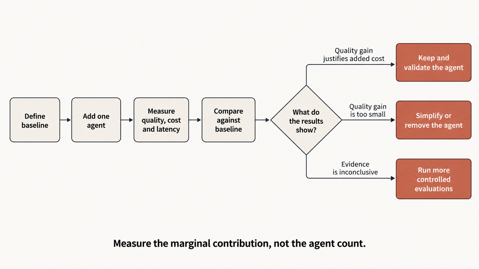
Published 25 October 2026 · Last verified 25 October 2026 · By the UniverseBlend editorial desk On 21 October, Meta set the latest marker for …
agentic AI

What Is Agentic AI? How AI Agents Work, What They Cost, and Where They Fail

Agentic AI describes software systems in which a language model chooses and carries out a sequence of actions to complete a task. It calls tools, …

AMD’s Hybrid AI Math: What the 40–60% Savings Model Assumes

Hybrid AI TCO

AMD says a fleet of 500 AI PCs running half their AI work locally can cost 40 to 60% less over three years than doing all of it through cloud APIs. The company built a calculator to show the arithmetic, which is more than most vendors do.

So the number is checkable. The question is what had to be true to produce it.

Run AMD’s Tokenomics Calculator at its defaults and three assumptions carry most of the weight: a daily token volume that only heavy agentic users reach, prompt caching switched off on the cloud side, and a local model whose quality the tool explicitly declines to compare. Change any one and the percentage moves substantially.

None of that makes the model dishonest. AMD discloses its assumptions more thoroughly than the headline suggests, including a frank exclusions list. But a modeled result under stated assumptions is not a property of hybrid AI, and the useful exercise for a buyer is working out which of those assumptions describe their own workload.

Key takeaways
  • The 40–60% figure is a modeled outcome for one scenario: 500 users at the Medium workload tier, 50% hybrid mix, three-year horizon, July 2026 cloud prices. It is not a general property of hybrid deployment.
  • The Medium tier assumes 5.74 million input and 574,000 output tokens per user per day — roughly 200 input tokens per second sustained across an eight-hour day. That is continuous agent activity, not assisted office work.
  • Prompt caching is supported in the calculator but off by default. Enabling it on a repetitive agentic workload can cut cloud input costs dramatically, which is the single biggest threat to the headline result.
  • At a 50% hybrid mix the calculator buys hardware for every user and runs half the tokens locally. The capital cost is full; the local utilisation is not.
  • AMD states plainly that the calculator does not consider performance needs and excludes model-quality differences, software licensing, IT management, migration, taxes, financing and egress.
  • Local throughput is measured on a quantised 35B open model. Comparing its cost against Claude Opus or GPT 5.5 pricing compares two different things.
  • The defensible conclusion: hybrid AI TCO can produce real savings for high-volume, repetitive, quality-tolerant workloads. Whether it does for you is a measurement question, not a percentage you can inherit.

Quick Navigation


What AMD’s Calculator Actually Models

Hybrid AI TCO is the total cost of running AI workloads across a mix of local hardware and cloud APIs, counting hardware, electricity and token charges over a defined period. AMD’s Tokenomics Calculator models three paths — cloud only, local on AMD devices, and a hybrid split — and reports three-year totals, monthly run rates and break-even months.

The inputs it takes:

InputOptions
Team size25, 250, 1,000 or custom
Analysis period1, 3, 4 or 5 years
Workload tierLight, Medium, Heavy or custom, as tokens per user per day
Cloud model mixGemini Pro $2/$12, Claude Sonnet $3/$15, Claude Opus $5/$25, GPT 5.5 $5/$30, or custom, per million tokens
Hybrid mix0% to 100% local
HardwareRyzen AI 9 HX 470, Ryzen AI Max+ 395, Radeon AI PRO R9700, with editable price, throughput, power and hours per day
EnergyElectricity rate and powered days per month
Cloud modifiersPrompt caching, batch discount, regional multiplier, long-context premium, monthly API surcharge

That is a more complete model than the headline implies, and the advanced panel exposes nearly every assumption for editing. Credit where it is due: the caching, batch and long-context controls exist, and most vendor calculators do not have them.

Three mechanics in the fine print matter more than anything on the main panel.

  1. Cloud cost is API tokens only. AMD states there is no seat, subscription or flat monthly price in the cloud figure. For an organisation actually paying per-seat for a coding assistant, this models a different cost structure than the one on their invoice — sometimes higher, sometimes lower.
  2. Hybrid buys hardware for everyone. At 50% mix, all users get a device and half the token volume runs on it. The hardware line is identical to a full local deployment.
  3. Hardware life equals the analysis period. Choose three years and the full device cost lands inside three years, adjusted by an end-of-life value percentage. There is no refresh cycle and no residual beyond that field.

AMD also prices local throughput from a specific measurement: Qwen 3.6 35B A3B at Q4_K_M quantisation, 262,000-token context prefilled to 128,000, sustained throughput under Vulkan llama.cpp. That is a real benchmark configuration, disclosed, and it is the quiet centre of the whole comparison — because it is the model whose cost is being compared against Claude Opus pricing.

The Token Assumption Does Most of the Work

5.74 million input tokens per user per day sounds abstract. Convert it and it stops being abstract.

Our calculations from AMD’s stated tier, using an eight-hour working day and 260 working days.

UnitInput tokensOutput tokens
Per day5,740,000574,000
Per hour (8h day)717,50071,750
Per second sustained~199~20
Per year~1.49bn~149m
Per 500-user fleet, per year~746bn~75bn

Two hundred input tokens per second, sustained, for every second of every working hour. That is not a person typing prompts. That is an agent running continuously, reading a repository, re-sending context and looping through tool calls.

For scale, 5.74 million tokens is in the region of four million words of input per person per day. No human reads or writes that. Only a machine loop produces it.

Three workload profiles, to show the spread. These are illustrative sketches, not measured data.

ProfileWhat it looks likeRough daily input tokens
Light office AIDrafting, summarising, occasional questionsTens of thousands to low hundreds of thousands
Knowledge worker with AI assistanceRegular use, document context, some retrievalHundreds of thousands to low millions
Continuous agentic codingCoding agent with large repo context, long sessionsMillions to tens of millions

AMD’s own Light tier sits at 574K input, a tenth of Medium. The gap between those two tiers is roughly the gap between a typical office deployment and a developer running a coding agent all day.

Why this dominates the result: cloud cost scales linearly with tokens while hardware cost is fixed. At the Medium tier on Claude Sonnet pricing, one user’s input tokens alone come to roughly $4,470 a year, with output adding about $2,240 — call it $6,700 per user per year, or $20,000 over three years. That is our arithmetic at AMD’s stated tier and prices. Against an AI PC costing one to three thousand dollars, the comparison is not close.

Drop to the Light tier and the same arithmetic yields roughly $670 per user per year. Now a $2,000 device takes about three years to pay for itself before counting electricity, management or anything AMD excludes, and the 40–60% headline does not survive.

The lesson is not that AMD picked an unfair number. It is that tier selection, more than hybrid mix, determines the answer. A buyer starting from the default tier rather than their own metered token volume is reading somebody else’s workload.

Where Prompt Caching Changes the Cloud Side

Here is the tension at the centre of the model. The workload that justifies the Medium tier — a continuous agent re-sending large context — is precisely the workload that prompt caching was designed for.

An agent turn is mostly repetition: the same system instructions, the same tool schemas, the same repository or document context, plus a small amount of genuinely new input. Providers price reused prefixes far below fresh input, and the discount is steep. On current frontier pricing, cached reads land near $0.20 per million tokens against input rates of $2 to $5. We worked through what that does to real bills in our analysis of the cache line that decides agentic costs.

AMD’s calculator supports this. The advanced panel has cache write share, cache read share, a write multiplier (1.25x for a five-minute window, 2x for an hour) and a read multiplier. The controls are there and they are correctly specified.

They are also off by default.

What that means in practice: the following is our illustrative arithmetic, not a calculator output. Take the Medium tier’s 5.74M daily input tokens on Claude Sonnet at $3 per million.

Cache-hit rateEffective input cost per user per dayAnnual input cost per user
0% (calculator default)$17.22~$4,477
50%$9.47~$2,462
80%$4.82~$1,253
90%$3.27~$850

At a 90% hit rate, the cloud input bill falls by roughly 80%. Since input dominates this workload’s token volume, that reshapes the entire comparison — and it reshapes it in the direction that hurts the local case.

The honest counterweight: high cache-hit rates are not automatic. They depend on prefix stability, on how the agent structures its context, on cache window duration against request frequency, and on provider implementation. An agent that rebuilds its context every turn gets little benefit and pays cache-write premiums for the privilege. Assuming 90% is as wrong as assuming zero.

So the correct criticism of AMD’s default is narrow and fair: for the specific workload profile that makes the Medium tier plausible, zero caching is the least likely assumption, and it is the one the tool ships with. Any buyer running this calculator should turn caching on and enter their own measured hit rate before reading the savings number.

The Utilisation Problem on the Local Side

The cloud side of this comparison is perfectly elastic: you pay for tokens consumed and nothing else. The local side is the opposite. You buy a device, and whether it earns its price depends entirely on how much work passes through it.

The calculator handles this more carefully than most. It has an “hrs/day running AI” field per device, it sizes capacity from throughput times that window, and it warns when fleet capacity falls short of token demand. Those are the right mechanics.

What the default scenario still implies is worth making explicit. At a 50% hybrid mix, every user gets a device and half the token volume runs on it. The device’s economic output is therefore half what the same hardware could produce — while its cost is unchanged. In utilisation terms, a 50% hybrid mix is a 50%-utilised fleet, at best.

Hybrid AI TCO

The gap between purchased and productive capacity has several sources, and they compound:

  • AI-active hours are not working hours. A device powered for eight hours may run inference for two.
  • One device per user caps sharing. The calculator states a hard ceiling of one device per user. A heavy user cannot borrow a colleague’s idle capacity.
  • Nights and weekends are free capacity nobody uses. Unless batch or background agent work is scheduled into them, two thirds of each day is idle.
  • Provisioning follows the peak. Hardware sized for the busiest user is over-provisioned for everyone else.
  • Adoption is uneven. Fleet-wide deployment assumes fleet-wide usage. Actual AI adoption inside organisations is famously lumpy.

This is the same economics we set out in our analysis of accelerator utilisation: once capacity is bought rather than rented, idle time stops being an efficiency question and becomes a cost-per-unit question. Every hour the device does not run inference raises the effective cost of the hours it does.

The flip side deserves equal weight, because it is the strongest argument for the local case. A device that runs background agents overnight, processes batch jobs on weekends, or serves a developer who genuinely saturates it can reach utilisation a cloud buyer pays dearly for. Local capacity has no marginal token cost. If you can fill it, you should.

The practical test is simple: measure AI-active hours per user, not headcount. A fleet where ten per cent of staff generate ninety per cent of token volume should not be deployed uniformly, and uniform deployment is exactly what the calculator’s hybrid model assumes.

The Missing Variable: Model Quality

AMD says this plainly, twice, and it deserves to be quoted rather than discovered: the calculator does not consider your performance needs, and model inference quality differences are excluded.

That exclusion is doing a lot of work, because of what is on each side of the comparison. The cloud column is priced from Claude Opus, GPT 5.5, Claude Sonnet or Gemini Pro. The local column is throughput-measured on Qwen 3.6 35B A3B at four-bit quantisation. Both are real. They are not the same capability, and the calculator compares their costs without comparing their outputs.

The economic principle is the one that matters here, and it generalises well beyond AMD:

Cost per token is not cost per completed task.

A cheaper model that needs more attempts can cost more in total. Work the chain through:

  • A task that takes two attempts instead of one doubles the token volume for that task
  • A task that needs human review consumes the most expensive resource in the building
  • A wrong output that reaches a downstream system costs far more than either
  • A longer reasoning path to the same answer burns more tokens on cheaper hardware

The arithmetic that follows is unforgiving. If a local model completes 70% of tasks that a frontier model completes at 95%, the effective cost per completed task rises by roughly a third before counting retries — and that is before anyone prices the human time spent on the failures.

None of this says local models are inadequate. Open models at 30B-class sizes have become genuinely capable, and for classification, extraction, summarisation, routing and structured transformation they are often indistinguishable from frontier models at a fraction of the cost. That is a real and growing category of work.

The point is narrower: a TCO model that excludes quality is answering “what does this cost?” rather than “what does this deliver per pound spent?” For the tasks where the two models are equivalent, AMD’s comparison is fair. For the tasks where they are not, the cost column is measuring the wrong thing — and the calculator cannot tell you which tasks are which. Only your own evaluation can.

Why 50/50 Is a Modeling Choice, Not a Strategy

The hybrid mix slider defaults to 50%. It is a reasonable midpoint for a demonstration and a poor description of how workloads actually divide.

Real routing is decided by task characteristics, not by percentages:

Route locallyRoute to cloud
Classification, extraction, taggingComplex multi-step reasoning
Summarisation of routine documentsNovel problem-solving
Privacy-sensitive or regulated dataTasks needing the newest model capabilities
High-volume repetitive transformationBurst workloads above local capacity
Offline or air-gapped workAnything where a wrong answer is expensive
Draft generation before human editingFinal output that ships unreviewed

Run that split against a real workload and the local share lands wherever it lands — 15%, 40%, 80%. The number is an output of the routing policy, not an input to it. An organisation doing mostly structured data work might route 80% locally. One doing mostly open-ended analysis might manage 20%.

This also explains why the calculator’s “max potential savings at 100% hybrid” figure should be read carefully. Full local means no access to frontier capability at all, which is a product decision rather than a cost optimisation.

What AMD’s Model Gets Right

Credit where it is earned, because the tool is better than the headline it generated.

  • It discloses its assumptions. Token tiers, model prices with a date, electricity rate, throughput test configuration, device specs — all visible and editable.
  • It publishes an exclusions list. Model quality, licensing, IT management, migration, taxes, financing, egress, volume discounts. Most vendor calculators omit this entirely.
  • It includes the modifiers that matter. Caching, batch discounts, long-context premiums and regional multipliers are all present, even if off by default.
  • It flags capacity shortfalls. If the fleet cannot serve the token demand, it says so and routes the overflow to cloud.
  • It states its own limitation on performance. “This calculator does not consider your performance needs” is an unusually honest sentence to put in a sales tool.
  • The underlying economics are sound. For sufficiently high, sufficiently repetitive token volumes, local inference genuinely is cheaper. That is not marketing; it is arithmetic.

What It Leaves Out That Could Matter

The exclusions are disclosed, but not all of them are equally consequential. Ranked by how much they could move a real result:

ExclusionWhy it mattersDirection
Model qualityChanges cost per completed task, not cost per tokenUsually favours cloud
Caching, when left offOverstates cloud input costs on repetitive workloadsFavours local as shipped
IT management and supportManaging local inference across a fleet is real workFavours cloud
Software licensingLocal serving stacks, management tooling, model licencesFavours cloud
Migration and deploymentOne-off but substantial for a 500-device rolloutFavours cloud
Hardware refreshLife is set to the analysis period; a 5-year window assumes 5-year devicesFavours local as shipped
Volume discountsEnterprise cloud agreements rarely pay list priceFavours cloud
Seat and subscription pricingMany organisations pay per seat, not per tokenDepends
Utilisation below 100%Capacity bought is not capacity usedFavours cloud

Notice the pattern. Most of the exclusions push in the same direction, and it is not the direction that makes local hardware look better.

A Better Hybrid AI TCO Calculation

Ten steps. The first four are measurement, and skipping them is how buyers end up with somebody else’s answer.

  1. Meter your actual token consumption. Pull it from provider dashboards or your gateway logs, not from headcount multiplied by an assumption.
  2. Separate input from output. They price differently and they scale differently. Input dominates agentic work; output dominates reasoning work.
  3. Measure your cache-hit rate. Most providers report cached-token usage. This single number may move your cloud bill more than any hardware decision.
  4. Measure AI-active hours per user, not working hours, and look at the distribution rather than the average.
  5. Classify tasks by quality requirement. Which actually need a frontier model? Test, do not assume.
  6. Calculate realistic local utilisation. Include nights, weekends and the users who barely touch AI.
  7. Add the omitted costs. Management, support, licensing, migration, refresh.
  8. Compute cost per completed task for both paths, including retries and human review.
  9. Test several routing mixes — 0%, 25%, 50%, 75%, 100% — rather than accepting the default.
  10. Run sensitivity on your two or three largest variables and see how wide the range gets.

Sensitivity: Which Assumptions Move the Answer

Directional, based on the model’s structure rather than on outputs we cannot reproduce exactly.

If this changesLocal and hybrid TCOWhy
Token volume risesImproves sharplyCloud scales linearly, hardware does not
Token volume fallsDeteriorates sharplyFixed hardware cost spread over less work
Cache-hit rate risesDeterioratesCloud input cost falls, sometimes by 80%+
Local utilisation risesImprovesSame capital, more output
Cloud API prices fallDeterioratesThe savings baseline shrinks
Electricity price risesDeteriorates mildlyPower is a small share at these volumes
Hardware price fallsImprovesLower capital to amortise
Quality requirements riseDeterioratesMore work must route to cloud regardless of cost
Refresh cycle shortensDeterioratesCapital amortised over fewer years
Hybrid mix rises toward 100%Improves on cost, narrows on capabilityFewer tokens billed, less frontier access

The two largest levers are token volume and cache-hit rate, and they pull in opposite directions on the same workload. That is the central tension in AMD’s model: the workloads with enough tokens to justify local hardware are the workloads most likely to benefit from caching.

FAQ

What is hybrid AI TCO?

The total cost of running AI workloads across both local hardware and cloud APIs over a defined period, counting hardware purchase, electricity and token charges. It differs from cloud-only TCO because part of the cost becomes fixed capital rather than metered usage.

Can hybrid AI really reduce AI costs by 40–60%?

AMD’s calculator produces that result for a specific scenario: 500 users at 5.74 million input and 574,000 output tokens per user per day, a 50% local mix, a three-year horizon and July 2026 cloud prices with prompt caching off. Under those assumptions the arithmetic holds. Whether it holds for a given organisation depends on whether its workload resembles that profile.

Is local AI cheaper than cloud AI?

For high-volume, repetitive, quality-tolerant workloads on well-utilised hardware, frequently yes. For light or intermittent usage, usually no, because fixed hardware cost is spread across too little work. The crossover point is set by token volume, utilisation and the cache-hit rate on the cloud side.

How does prompt caching affect hybrid AI TCO?

Significantly, and against the local case. Cached input tokens are priced far below fresh ones, so a repetitive agentic workload with a high hit rate can cut its cloud input bill by most of its value. AMD’s calculator supports caching but ships with it disabled, which prices every input token at full rate.

How much does AI PC utilisation affect TCO?

Proportionally. A device used half as much has roughly double the effective cost per unit of work, since the purchase price does not change. At a 50% hybrid mix the calculator buys hardware for every user and runs half their tokens locally, which is a 50%-utilised fleet by construction.

What costs are missing from AMD’s AI cost calculator?

AMD lists them: model inference quality differences, software licensing, IT management, migration effort, taxes, financing fees, network and egress costs unless entered manually, and provider-specific volume discounts. Most of these, if included, would favour the cloud side.

Is a 50/50 local and cloud split optimal?

It is a default, not an optimum. The right mix follows from task routing — which work genuinely needs frontier capability and which does not — and lands anywhere from 15% to 80% local depending on the workload.

How should businesses calculate AI TCO?

Start by metering actual token consumption split into input and output, measure the cache-hit rate and AI-active hours per user, classify which tasks need frontier models, then compute cost per completed task for several routing mixes rather than cost per token for one.

Does AMD’s calculator compare equivalent models?

No, and it says so. Local throughput is measured on Qwen 3.6 35B A3B at four-bit quantisation, while cloud costs are priced from Claude, GPT and Gemini models. AMD states explicitly that the tool does not consider performance needs.


Keep reading

Kimi K3.1 Pro

Kimi K3.1 Pro vs Sonnet 5.5: Same Price, Different Bill

On paper, Moonshot AI priced Kimi K3.1 Pro to the cent against Claude Sonnet 5.5: $2 per million input tokens and $10 per million output …
RAG vs fine-tuning

RAG vs Fine-Tuning: Which One You Actually Need

Take a support team that ships two prototypes on the same base model. The first searches the product documentation on every question and pastes the …
AI capex

AI Infrastructure Spending: What $145 Billion and a Sold-Out AWS Actually Buy

Published 25 October 2026 · Last verified 25 October 2026 · By the UniverseBlend editorial desk On 21 October, Meta set the latest marker for …
agentic AI

What Is Agentic AI? How AI Agents Work, What They Cost, and Where They Fail

Agentic AI describes software systems in which a language model chooses and carries out a sequence of actions to complete a task. It calls tools, …

Gemini Free Plan Drops to Flash-Lite Only on October 9

Gemini Free Plan

If you use Gemini without paying, the model picker is about to get shorter. On October 9, 2026, the Gemini Free Plan stops offering Flash and Pro in the Gemini app and keeps one model: Flash-Lite.

That is not a rumor. Google’s own support page lays it out. What the page leaves out is why Google is doing it and how different the answers will feel. Headlines have filled that gap with words like “downgrade,” which tells you how people feel but not what to do.

The more useful question is this: if your daily routine runs on free Gemini, which parts of it were quietly leaning on the bigger models? This article separates what Google has confirmed, what has only been reported, what I am inferring, and what nobody outside Google knows yet.

Key takeaways
  • Confirmed: from October 9, 2026, the Gemini Free Plan in the Gemini app offers Flash-Lite only.
  • Confirmed: AI Plus keeps Flash-Lite and Flash but loses Pro, on an account-specific date sent by email.
  • Not a quota change: it is a model-access change, layered on top of the compute-based limits that began May 17.
  • Likely to matter most for complex reasoning, bigger coding jobs and multi-source research.
  • Likely to matter least for summaries, quick questions, translation and routine writing.
  • Inferred, not stated: cost and capacity pressure sits behind the move. Google has not said so.
  • API and AI Studio: nothing found suggests they are affected, but verify before you rely on that.

Quick Navigation


What the Gemini Free Plan Change Actually Is

Google’s help page, “Changes to Gemini model access and limits,” says model availability in Gemini Apps changes for personal accounts starting in October 2026. For people without an AI subscription, the change takes effect on October 9. After that, an account with no plan gets Flash-Lite. Flash and Pro are removed.

Two details are easy to miss. First, “Gemini Free Plan” is a reader-friendly phrase, not Google’s label. The page says “without a plan.” Second, this is not only a free-tier story. Google AI Plus subscribers keep Flash-Lite and Flash but lose Pro, on a date Google says it will send by email. AI Pro and AI Ultra keep all three.

Here is how the evidence breaks down:

StatusWhat we know
Confirmed (Google support page)Applies to Gemini Apps on personal accounts. Free: Flash-Lite only from October 9. AI Plus: Flash-Lite and Flash. AI Pro and Ultra: all three. Low, medium and high effort levels for each model. Deep Think for AI Pro and Ultra.
Reported (9to5Google and others)Versions are 3.5 Flash-Lite, 3.6 Flash and 3.1 Pro. US prices are $4.99 for AI Plus and $19.99 for AI Pro. Deep Think was previously limited to the $99.99 and $199.99 plans.
Inferred (my analysis)Compute cost and capacity are part of the motive. The new ladder nudges free users toward paid plans.
UnknownGoogle’s stated reason, exact Flash-Lite limits, rules for work or school accounts, and rollout differences by country.

Flash-Lite Is a Model, the Gemini Free Plan Is an Access Tier

The key distinction: Flash-Lite is a model. It is the smallest of three tiers in the Gemini family, alongside Flash and Pro. The Gemini Free Plan is a level of access to the Gemini app. Plans decide which models you can open and how much you can use them.

Mixing these up causes real confusion. “Google AI Pro” is a subscription. “Gemini Pro” is a model. Saying Google “removed Pro” is only true if you specify which plan.

This change is about model availability, not a quota tweak. Quotas are a separate layer. Since May 17, 2026, the Gemini app has used compute-based limits that refresh every five hours until you hit a weekly cap. Google says usage depends on prompt complexity, the features you use and chat length. Paid plans get higher allowances: AI Plus 2x the standard limit, AI Pro 4x, and Ultra 5x or 20x higher than Pro.

So October 9 adds a second gate on top of the first. One gate decides which models you can open. The other decides how much you can use them.

A note on version numbers. Google’s help page uses family names only. The version labels come from 9to5Google’s reporting, and some trackers already list newer Flash builds. Check what your own picker shows.

What Flash-Lite Is Built to Do

Google released Gemini 3.5 Flash-Lite on July 21, 2026, alongside 3.6 Flash. It is aimed at high-volume, low-latency work such as search-style tasks and document processing. Google says it is a clear step up from the March 3.1 Flash-Lite.

Gemini Free Plan

In the API, it is priced at $0.30 per million input tokens and $2.50 per million output tokens. Artificial Analysis lists a roughly one-million-token context window, with text, image, speech and video input and text output. Google’s own benchmark claims compare it with its predecessor and with the older Gemini 3 Flash. For example, it scores 54.2% against 49.6% on SWE-Bench Pro versus that older model. These are vendor-reported numbers.

In plain English, Flash-Lite is the fast, cheap model. It is built for volume, not for your hardest problem of the week. One caution: those specs are API specs. I found no published documentation of per-model context or file limits inside the Gemini app, so don’t assume the app matches.

The Workloads Where Gemini Free Plan Users Will Notice It

No one has published a side-by-side test of Flash-Lite against 3.6 Flash or 3.1 Pro on everyday app tasks. This table is my editorial judgment based on how Google positions the models. It is not test data.

WorkloadLikely impactWhy
Complex multi-step reasoningHighPro was the heavyweight option, and Flash-Lite is tuned for speed and volume
Larger coding tasksModerate to highGoogle reports strong coding gains, but longer refactors lean on bigger models
Research across several sourcesModerateSynthesis and judgment are where lighter models tend to thin out
Long-document analysisModerateThe context window is large on paper, and Google reports better long-context scores than its predecessor, but app limits are undocumented
Multimodal tasksUnclearThe model accepts images, audio and video, but there is no app-level comparison
Basic writing and editingLow to moderateFine for drafts, though nuance and tone may be flatter
Simple summaries, translation, quick questionsLowClose to what the model was built for
Repetitive everyday promptsLowSpeed helps here

The pattern is simple. The more a task needs the model to hold several ideas at once and reason through them, the more the gap will show. Google does offer a partial remedy. Each model gets low, medium and high effort levels, and higher effort means more thorough answers but uses more of your limit. A free user can push Flash-Lite harder, but will probably run out sooner.

The Workloads Where You Probably Won’t

Many free users will barely notice. Summarizing a PDF, rewriting an email, planning a trip, explaining a concept or checking a homework answer are tasks a lightweight model can handle well. Speed is a real benefit there.

There is one catch. Reports based on Google’s plan pages say the free app currently defaults to Flash. If that is right, the default experience changes even for people who never opened the picker. Those people won’t know a switch happened. They will just find answers thinner on harder questions.

Is Flash-Lite Actually Worse?

Not in a simple way. “Less capable for some workloads” does not mean “bad.” A model that answers in two seconds with a decent summary can beat a heavier model that takes longer, especially for routine work.

Benchmarks help only a little here. Google’s published numbers compare Flash-Lite with its own predecessor and an older Flash, not with the models free users are losing. I could not find an apples-to-apples comparison against 3.6 Flash or 3.1 Pro. Even if one existed, benchmark scores would not predict whether your essay outline or spreadsheet formula comes out right. The only reliable test is your own prompts.

Why Google Would Make This Trade-Off

  • What Google states: nothing, at least on the support page. It announces the change without explaining it.
  • What Google’s own page implies: it lists the Pro model, Deep Think, extended thinking, media generation and Deep Research as things that use more of your limit. That is Google describing which features cost more to run.
  • What I infer: inference economics. Every response costs compute, and free users generate a lot of volume with no direct revenue. API list prices offer a rough proxy. Flash-Lite lists at $0.30 and $2.50 per million tokens, against $1.50 and $7.50 for 3.6 Flash. That is five times on input and three times on output. List price is not Google’s internal cost, but the direction is clear. For a deeper look at how token costs compound, see UniverseBlend’s Cluster Topology Decides What You Can Actually Run.

There is also a ladder effect. AI Plus loses Pro, and AI Pro gains Deep Think. That makes AI Pro the cheapest plan with all three models, which looks like a repricing of the tiers. Whether it is designed as an upsell, Google has not said. Google also announced Gemini 4 Argon on September 30, first for AI Ultra. Nothing I found links that to this change.

Free vs Paid: Where the Gemini Free Plan Line Now Sits

PlanUS price (reported)ModelsUsage limit
No plan$0Flash-LiteStandard
Google AI Plus$4.99/monthFlash-Lite, Flash2x standard
Google AI Pro$19.99/monthFlash-Lite, Flash, Pro, Deep Think4x standard
Google AI Ultra$99.99 or $199.99/monthAll three, Deep Think5x or 20x AI Pro

Prices vary by country, so check the figure in your own app. The practical shift is for AI Plus. It is now the middle step that stops short of Pro. If you needed Pro regularly, Plus will not solve it.

Gemini API and AI Studio: What Developers Need to Know

Google’s support page covers Gemini Apps on personal accounts. It does not mention the Gemini API or Google AI Studio, and I found no evidence that either is part of this change. Independent trackers say the API still has a free tier for eligible models as of October 1, with limits that vary by model and project. They also report that 3.1 Pro Preview is paid-only there.

The practical lesson is to treat the consumer app and the API as separate products. If you have been using the app as a testing bench, an API key gives you control over which model runs. Free-tier API prompts may also be used to improve Google’s products, so keep client or sensitive data off it. And since models change under you, UniverseBlend’s piece on What Breaks When Your Model Version Retires is a useful checklist.

The Unanswered Questions

  • Why Google made the change, in its own words.
  • What the real Flash-Lite limits are in the app, including whether it still counts against the five-hour and weekly caps. One report cites an in-app popup promising continued unlimited access, but the support page I read does not say that.
  • How work and school accounts are treated.
  • Whether the rollout is staggered by country or age, as the May changes were for under-18 users.
  • Where Gemini 4 Argon fits in the plan structure.

What I Would Do as a Gemini Free Plan User

First, finish anything that depends on Flash or Pro before October 9, and save the outputs. Second, pick your five most-used prompts and run them on Flash-Lite as soon as it is your only option. Note which ones fail, because that list is your real upgrade case.

Third, use effort levels deliberately. Start low, and raise effort only when the answer is thin. Fourth, break big tasks into smaller steps and verify anything that matters, since lighter models are more likely to skim.

On paying: if your failures are occasional, stay free. If you need Pro weekly, AI Pro is the cheapest plan that includes it. If you are a developer, test through the API before paying for the app. I have not tested Flash-Lite myself for this article, so treat this as a planning approach, not a verdict.

FAQ

What is changing in the Gemini Free Plan on October 9?

Free users lose Flash and Pro in the Gemini app and keep only Flash-Lite. The change applies to personal accounts, and Google confirms it on its support page. AI Plus subscribers also lose Pro, on their own schedule.

Is Gemini Flash-Lite free?

Yes, Flash-Lite stays available in the Gemini app without a subscription. In the API, many Flash-family models have a free tier, but check Google’s current pricing table for the specific model ID, since limits change.

Is Gemini Flash-Lite less capable than Gemini’s larger models?

Generally yes, by design. It is Google’s fastest and cheapest tier. No published comparison shows exactly how much weaker it is on everyday app tasks.

Will Gemini Free users lose access to advanced models?

In the app, yes: Flash and Pro both go. Pro and Deep Think remain on paid plans, with Deep Think available on AI Pro and Ultra.

Does the change affect the Gemini API or Google AI Studio?

Nothing Google published says so. The support page covers Gemini Apps on personal accounts only. Check the API pricing and rate-limit pages directly.

Should I upgrade from Gemini Free?

Only if Flash-Lite fails your real prompts. AI Plus adds Flash, while AI Pro is the cheapest plan that keeps all three models and adds Deep Think.

Is Gemini still worth using for free?

For lighter work, yes. For heavy reasoning or complex coding, expect to feel the limits.

What is Gemini Flash-Lite?

It is the smallest model in Google’s Gemini family, built for fast, high-volume tasks like summarizing and document processing. Version 3.5 launched on July 21, 2026.


Keep reading

Kimi K3.1 Pro

Kimi K3.1 Pro vs Sonnet 5.5: Same Price, Different Bill

On paper, Moonshot AI priced Kimi K3.1 Pro to the cent against Claude Sonnet 5.5: $2 per million input tokens and $10 per million output …
RAG vs fine-tuning

RAG vs Fine-Tuning: Which One You Actually Need

Take a support team that ships two prototypes on the same base model. The first searches the product documentation on every question and pastes the …
AI capex

AI Infrastructure Spending: What $145 Billion and a Sold-Out AWS Actually Buy
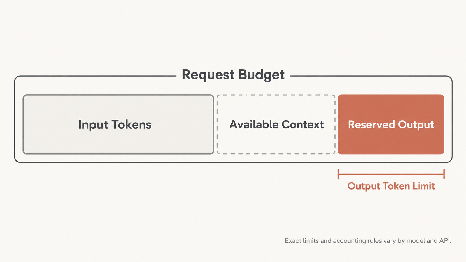
Published 25 October 2026 · Last verified 25 October 2026 · By the UniverseBlend editorial desk On 21 October, Meta set the latest marker for …
agentic AI

What Is Agentic AI? How AI Agents Work, What They Cost, and Where They Fail

Agentic AI describes software systems in which a language model chooses and carries out a sequence of actions to complete a task. It calls tools, …

Anthropic’s $518B Compute Commitment: The Obligation Behind It

Anthropic compute commitments

The number everyone repeated last week was $518 billion. The number that actually matters is 80%.

That is the share of Anthropic’s future compute and infrastructure commitments described as non-cancelable or payable regardless of usage, according to a confidential IPO prospectus reviewed by Reuters. Strip out the second number and the first is just a large purchase order from a company that needs a lot of chips. Keep it, and the commitment changes category: from a plan to spend into an obligation to pay.

Those are different things, and the difference is the whole story.

Having access to compute solves what has been the binding constraint on frontier AI development for three years. Being contractually obligated to pay for compute, on a schedule set in advance, converts a supply problem into a utilisation problem — and utilisation is something a company controls only partly, because it depends on customers showing up on the timetable the contracts assumed.

Key takeaways
  • A confidential IPO prospectus reviewed by Reuters shows Anthropic committed to at least $518 billion over roughly a decade across six infrastructure partners, with about 80% non-cancelable or payable regardless of usage.
  • The largest reported components: approximately $161.2bn in Broadcom-related equipment leases, $111.1bn with Google, $110bn with Amazon, $31.4bn with Microsoft, about $84.5bn for Nvidia-based capacity and about $20bn with AMD.
  • The commitments are not uniform. Reporting describes shortfall payments for Google and Amazon, cancellation only on uncured material breach for Microsoft, and leases cancelable only on default for Broadcom. One percentage covers four different contract types.
  • Anthropic spent $7.33 billion on compute and infrastructure in 2025 — more than half of $12.65 billion in total operating expenses — against revenue of $4.59 billion and $20.28 billion of cash and short-term investments.
  • Broadcom has reportedly agreed to lend up to $42 billion through a convertible note that could fund about a third of a five-year, $125.2 billion TPU lease, making one company supplier, lessor and lender at once.
  • Long-term commitments buy capacity certainty in a market where capacity has been the constraint. The cost of that certainty is financial rigidity if demand arrives later or smaller than contracted.
  • The exact terms remain unverifiable while the prospectus is confidential. That uncertainty is part of the story, not a gap in it.

Quick Navigation


What the $518 Billion Actually Represents

Anthropic’s compute commitments are contractual obligations to buy cloud services, computing capacity and AI infrastructure from named partners over a defined period. They are not a debt balance, not a cash payment, and not a single contract.

The reported breakdown, all from the prospectus as described by Reuters:

PartnerReported amountWhat it coversPeriod
Broadcom~$161.2bnEquipment lease obligations, largely non-cancelableIncludes a five-year TPU capacity lease of $125.2bn
Google~$111.1bnInfrastructure servicesApril 2026 – July 2033
Amazon$110bnInfrastructure servicesMay 2026 – April 2036
Nvidia-based capacity~$84.5bnCompute capacityThrough 2029
Microsoft$31.4bnInfrastructure servicesNovember 2026 – May 2033
AMD~$20bnAI computeNot reported

Those six figures sum to roughly $518 billion, which matches the headline. Note the composition: the single largest line is not a cloud contract at all but equipment leases, which behave differently from service agreements in both accounting and cancellation terms.

Three distinctions matter before anyone compares this to a balance sheet.

  1. Commitment is not cash. A ten-year obligation is paid over ten years. Spread evenly — which it will not be, since these ramp — $518 billion is roughly $50 billion a year, against the $7.33 billion Anthropic actually spent on compute and infrastructure in 2025.
  2. Commitment is not debt. It does not sit on the balance sheet as borrowing, though lease obligations are capitalised under current accounting. It is a future purchase obligation, disclosed in the commitments note rather than counted as leverage.
  3. The period is long and the ramp is steep. Contracts running to 2033, 2036 and beyond assume a company much larger than today’s. Reuters reported an annualised revenue run rate above $65 billion by the end of July and earlier reporting put Anthropic’s own 2028 revenue projection at roughly $190–200 billion. Those projections are the company’s, not forecasts anyone has validated.

The useful comparison is not $518 billion against $4.59 billion of 2025 revenue — that ratio is dramatic and tells you almost nothing. It is annual contracted spend against annual revenue in each future year, which is where the question of whether the commitments are comfortable or binding actually gets settled.

The Obligation Hidden Inside the Headline

The 80% figure is a summary statistic covering several different contractual mechanisms, and the mechanisms matter more than the average.

From the reporting:

  • Google and Amazon: Anthropic must pay the difference if its actual spending falls short of the minimum commitment. This is a shortfall provision — you can buy less, but you pay the same.
  • Microsoft: the agreement is described as non-cancelable through May 2033 absent an uncured material breach.
  • Broadcom: the equipment leases are largely non-cancelable except after default, and certain payment or performance defaults could make a substantial portion of the lease obligations immediately payable.
  • The Nvidia-based capacity arrangement: described as giving Anthropic more room to retreat than the others.

So “80% non-cancelable” bundles a minimum-volume commitment, a breach-only termination clause, a lease default provision and at least one more flexible arrangement under a single number.

That distinction has a practical consequence. A shortfall provision caps your downside at the committed spend — you lose the optionality, not more. A lease acceleration clause is different in kind: default can pull future payments forward into the present, which turns a long-dated obligation into an immediate one at exactly the moment a company would least be able to meet it.

The prospectus itself flags this. Reporting describes a warning that certain defaults could accelerate a substantial portion of lease obligations while also restricting Anthropic’s ability to draw on the $42 billion Broadcom facility to cover them. A financing facility that becomes unavailable precisely when it is needed is a standard credit structure and a real risk factor.

What cannot be verified: the actual contract language, the ramp schedules, the definitions of “minimum commitment”, any price-adjustment or technology-refresh provisions, and whether the agreements contain renegotiation mechanisms that reporting has not described. The prospectus remains confidential. Anyone asserting precision about these terms is working from the same journalism everyone else is.

Take-or-Pay Changes the Utilisation Equation

Take-or-pay means the buyer pays for a contracted quantity whether or not it takes delivery. The structure comes from energy and shipping, where suppliers build expensive dedicated capacity and need revenue certainty to justify it. It is appearing in AI infrastructure for exactly the same reason: someone has to fund the data centre before the demand shows up.

For the buyer, take-or-pay converts a variable cost into a fixed one. That is the entire economic consequence, and it cuts both ways.

Anthropic compute commitments

Here is what it does to the unit economics. The following is a hypothetical illustration, not a description of any Anthropic contract or price.

Suppose a company commits to $10 billion of compute capacity for a year under a take-or-pay arrangement.

ScenarioCapacity usedCost incurredEffective cost per unit used
Demand as planned100%$10bn1.0x
Demand arrives late70%$10bn1.43x
Demand disappoints50%$10bn2.0x
Usage-based contract, same shortfall50%$5bn1.0x

Under a usage-based contract, a demand shortfall is a revenue problem. Under take-or-pay, the same shortfall is a revenue problem and a margin problem, because the denominator shrinks while the numerator does not.

This is why utilisation stops being an engineering concern and becomes a financial one. When capacity is elastic, running accelerators at 60% is an optimisation question — you are leaving efficiency on the table. When capacity is committed and paid for regardless, 60% utilisation means 40% of a contracted dollar produced nothing, and that gap flows directly into gross margin. We worked through the mechanics of where idle capacity comes from in our analysis of accelerator utilisation, and every source of idle time in that piece becomes more expensive under this contract structure.

The pressure this creates is directional and predictable. A company with committed capacity has strong incentives to fill it: push inference volume, expand enterprise contracts, launch workloads that consume compute, price aggressively to drive usage. None of those are irrational responses. They are what the contract structure rewards.

The honest caveat: none of this establishes that Anthropic is underutilising anything. Its reported run-rate growth suggests demand has been the easier half of the equation so far. The point is structural — take-or-pay raises the cost of being wrong about timing, for anyone who signs it.

Why Compute Certainty Can Be Worth Paying For

It would be easy to write this as a cautionary tale. That reading ignores why a competent management team signs these contracts, and the reasons are good ones.

For the past three years, the binding constraint on frontier AI has been access to compute, not demand for it. Accelerators have been allocated rather than sold. Memory has been contracted years ahead. Data-centre power has become a multi-year procurement problem. In that environment, a company without secured capacity does not get to choose how fast it grows.

What a long-term commitment buys:

  • Capacity that exists. Suppliers build against contracted demand. An uncommitted buyer competes for whatever is left.
  • Price certainty in a rising market. If compute costs rise, a fixed contract becomes an asset. The hedge runs both directions.
  • Planning horizon. Model development schedules depend on knowing what hardware will be available and when.
  • Priority on new generations. Being a large committed customer affects allocation when the next accelerator ships short.
  • Scale economics. Volume commitments buy better unit pricing than spot purchasing.

There is also a competitive dimension. If frontier capability tracks compute, then capacity secured is capability secured, and capacity your competitor cannot buy is capability they cannot build. Commitments of this size take supply off the market.

The trade-off is clean enough to state in one sentence: Anthropic has exchanged financial flexibility for compute certainty. Whether that was a good trade depends entirely on which constraint turns out to bind — and that will not be clear for years.

The Partners Behind the Anthropic Compute Commitments

The prospectus, as reported, identifies Amazon, Google and Microsoft as simultaneously investors, customers, cloud providers, distributors and competitors. That is not a conflict the company is hiding; it is one it is disclosing as a risk.

Each role pulls differently. As an investor, a partner benefits from Anthropic’s success. As a supplier, it benefits from Anthropic’s spending. As a distributor, it takes a margin on Anthropic’s models. As a competitor, it builds models that compete with them. The same counterparty occupies all four positions at once.

The Broadcom structure is the sharpest version. Reuters reported on October 1 that Broadcom agreed to lend Anthropic up to $42 billion through a convertible note that could fund roughly a third of the five-year, $125.2 billion TPU compute lease, with Broadcom permitted to designate a financing partner and the debt convertible into Anthropic equity. Anthropic is expected to become the largest customer in Broadcom’s chip design business next year.

So one company supplies the hardware, leases it, lends the money to pay for the lease, and may end up holding equity. The prospectus reportedly flags potential conflicts of interest directly, warning that Broadcom’s decisions on pricing and hardware could affect Anthropic’s ability to procure enough computing infrastructure.

Broadcom’s own public filings describe a structure of this shape without naming a customer. Its 10-Q for the quarter ended August 2, 2026 discloses an “AI XPV platform” launched in June 2026 with an initial $35 billion tranche led by a financial partner, enabling deployment of more than a gigawatt of compute infrastructure for a customer, with Broadcom providing a backstop on that customer’s five-year lease obligations and maximum potential liability of roughly $29 billion. Broadcom does not identify the customer, and no public source establishes that these are the same arrangement.

The economic observation, offered as analysis: vendor financing linked to future demand for the vendor’s own product is not new — it is how equipment vendors have supported large customers for decades, and Nvidia has done versions of it recently. What is different here is the concentration. The same relationship carries supply risk, credit risk and equity exposure, and a stress event in one leg propagates to the others. Rothschild’s Robert Leitao put the market’s version of this concern plainly, questioning whether the revenue base can keep pace with the scale of financing that has been arranged.

Leases, Depreciation and the Technology Risk in a Long Contract

Three concepts get conflated whenever AI infrastructure costs come up, and they are related but not interchangeable.

ConceptWhat it isWhere it shows up
Contractual commitmentA promise to buy capacity or services in future periodsCommitments note; lease liabilities on the balance sheet
DepreciationAllocation of an owned asset’s cost across its useful lifeOperating expenses, for hardware you own
Operating expenseCash cost of running the business in a periodIncome statement

For a company leasing capacity rather than buying accelerators, depreciation largely sits with whoever owns the hardware — but the economics do not disappear. They arrive embedded in the lease rate, because the lessor priced in the asset’s expected useful life when setting it.

That is where the technology risk lives. A five-year lease on a specific accelerator generation assumes that generation stays economically competitive for five years. Hardware improves on a roughly annual cadence now, and what ends an accelerator’s economic life is usually not failure but the arrival of something that does more per watt and holds more memory — the pattern we examined in our piece on AI accelerator depreciation.

Follow that through. If performance per dollar improves sharply in 2029, a lease signed in 2027 at 2027 rates becomes expensive relative to what the market then offers. The capacity still works. It is simply worth less than it costs, and the contract does not care.

This is the structural reason long compute contracts carry risk that long property leases do not. A building is still a building in year seven. An accelerator generation may be two or three generations behind by then, and the memory capacity that made it viable for a given model size may no longer fit the models being served.

The counterweight, in fairness: the TPU capacity in question reportedly starts coming online in 2027 and the lease runs five years from there, which is roughly in line with how hyperscalers depreciate their own fleets. These are not exotic terms. They are standard terms applied at an unusual scale, and the scale is what makes the technology-refresh assumption consequential.

What Could Make the Anthropic Compute Commitments Work

The bull case is not complicated, and it is mostly about one variable arriving on schedule.

If enterprise AI demand grows as projected, contracted capacity gets consumed, and the commitments look like foresight rather than exposure. Reuters reported an annualised revenue run rate above $65 billion by the end of July, against $4.59 billion for full-year 2025. A company growing at that rate does not have a utilisation problem; it has a capacity problem, which is what the contracts solve.

Several things reinforce that outcome:

  • Compute stays scarce. If accelerators, memory and power remain constrained, fixed-price contracts signed earlier look cheap later.
  • Agentic and reasoning workloads consume more per task. Demand per customer rises without needing more customers.
  • Enterprise contracts lengthen. Multi-year customer commitments on the revenue side offset multi-year obligations on the cost side, which is the natural hedge.
  • Scale lowers unit cost. Large committed volumes buy better pricing than anyone purchasing on demand.

The cleanest version of the bull case: the commitments convert an unpredictable supply risk into a predictable cost, in a business where supply has been the thing that limited growth.

What Could Make Them Expensive

The bear case does not require AI demand to collapse. It only requires the economics of compute to move faster than the contracts.

  • Efficiency improves faster than demand grows. Better quantisation, more efficient architectures and cheaper serving reduce compute per unit of output. The same revenue then needs less capacity, and contracted capacity goes unused.
  • Performance per dollar jumps. A new accelerator generation that is substantially more efficient makes older contracted capacity expensive relative to what is available, exactly as described above.
  • Price competition compresses margins. If model API prices keep falling — and they have fallen steeply — revenue per unit of compute falls with them, while the cost per unit is fixed by contract.
  • Demand arrives late rather than never. This is the underrated scenario. Contracts ramp on a schedule. If adoption lands two years behind the schedule, the capacity is paid for during the gap.
  • Customer concentration bites. Reporting indicates two customers supplied nearly a quarter of 2025 revenue. Concentrated revenue against distributed fixed obligations is an asymmetry worth noting.
  • Capital markets tighten. Much of this structure assumes continued access to financing, including the Broadcom facility. The prospectus reportedly warns that certain defaults could both accelerate lease obligations and restrict access to that facility.

None of these is a prediction. They are the variables that would determine whether a commitment of this size reads as strategic or as overextended, and they are the ones worth tracking.

The Valuation Connection

A valuation above $2 trillion — against a self-estimated $965 billion in May — is a statement about future cash flows. Those cash flows depend on revenue growth, gross margin, capital intensity and how much compute each dollar of revenue requires.

What the $518 billion does is make one of those variables visible. Infrastructure spending is normally a forecast assumption that investors argue about. Here, a large portion of it is contracted, dated and disclosed. The spending is no longer a question mark; what remains uncertain is the revenue that has to arrive alongside it.

This is not an argument that the valuation is right or wrong, and this article offers no view on that. The structural observation is narrower: when costs are contractually fixed and revenues are not, the equity absorbs the variance. That is true of any capital-intensive business, and it is unusual to see it at this scale in a company five years old.

The 2025 figures give a sense of the starting point. Revenue of $4.59 billion, operating loss of $8.06 billion, compute and infrastructure spending of $7.33 billion within $12.65 billion of total operating expenses, and $20.28 billion of cash and short-term investments at year end. The headline $42 billion net loss is mostly a non-cash charge of roughly $34 billion tied to the rising estimated value of convertible financing instruments — a number that grows precisely because the company’s valuation grew, and which tells you nothing about operations.

A Note on Governance

Briefly, because it is a separate question from the economics.

Reporting describes a newly created “Founder LLC” comprising Anthropic’s seven co-founders, holding a single Class F share carrying 50.1% of voting power on certain matters including some director elections. The founders direct that share by majority vote. The structure is not permanent: a founder who leaves, dies, sells below a threshold or is removed for cause drops out, and the super-voting class begins to sunset once few enough founders remain.

That is the factual position. Dual-class structures are common in technology listings, and whether this one is appropriate is a judgement for investors rather than for this article. The relevant connection to the rest of the piece is simply that financial scale and governance structure are independent: the commitments would have the same economics under any voting arrangement.

What AI Infrastructure Buyers Should Take From This

Most organisations will never sign a contract with nine zeros. The structural lessons scale down anyway.

  • Know which of your compute spend is committed. Reserved instances, savings plans, minimum commitments and capacity reservations all behave like small take-or-pay contracts. The percentage of your bill that is committed is the percentage where utilisation becomes a margin issue.
  • Model the shortfall, not just the spend. The question is not what the commitment costs. It is what it costs if you use 60% of it.
  • Match contract duration to demand visibility. A three-year commitment against six months of demand visibility is a bet, however good the discount.
  • Price the flexibility you are selling. Vendors discount committed volume because certainty is worth something to them. Work out what it is worth to you before trading it away.
  • Watch counterparty concentration. If the same vendor supplies, finances and distributes, your exposure to them is larger than any single contract suggests.
  • Treat utilisation as a financial metric. Once capacity is committed, the operations team’s efficiency work shows up in gross margin. That changes who should be in the room when it is discussed.

The question this story leaves open is a genuine one. Does committing $518 billion remove Anthropic’s biggest risk — not being able to get compute — or substitute a different one, being obligated to pay for compute whether or not demand arrives on schedule? The answer is that it does both, and which dominates depends on variables that will take years to resolve: utilisation, revenue growth, contract terms nobody outside has seen, compute prices, model efficiency and how quickly hardware generations turn over.

Anyone offering a confident verdict today is working from the same confidential document nobody has read.

FAQ

What are Anthropic’s compute commitments?

Contractual obligations to purchase cloud services, computing capacity and AI infrastructure from named partners over fixed periods. According to a confidential IPO prospectus reviewed by Reuters, they total at least $518 billion over roughly a decade across six partners.

What is the $518 billion figure?

The sum of Anthropic’s disclosed infrastructure commitments: approximately $161.2bn in Broadcom-related equipment leases, $111.1bn with Google, $110bn with Amazon, about $84.5bn for Nvidia-based capacity, $31.4bn with Microsoft and about $20bn with AMD. It is a multi-year obligation, not a current debt or a cash payment.

What does take-or-pay mean here?

That the buyer pays for contracted capacity whether or not it is used. Reuters reported that about 80% of Anthropic’s commitments are non-cancelable or payable regardless of usage, though the specific mechanisms differ by counterparty.

What happens if Anthropic does not use the contracted compute?

Based on the reported terms, it would still owe the money in most cases — through shortfall payments to Google and Amazon, or through lease obligations to Broadcom. The exact provisions cannot be verified while the prospectus stays confidential.

Why would a company commit so much compute?

Because compute availability, not demand, has been the binding constraint on frontier AI development. Long-term commitments secure capacity, lock in pricing, support planning and give priority on new hardware generations — at the cost of financial flexibility.

Who provides Anthropic’s compute?

Six partners per the reported prospectus: Broadcom, Google, Amazon, a provider of Nvidia-based capacity, Microsoft and AMD. Amazon, Google and Microsoft are described as simultaneously investors, customers, cloud providers, distributors and competitors.

What is the Broadcom financing arrangement?

Reuters reported that Broadcom agreed to lend Anthropic up to $42 billion via a convertible note that could fund roughly a third of a five-year, $125.2 billion TPU compute lease. Broadcom may designate a financing partner, and the debt could convert into Anthropic equity.

How do compute commitments affect AI company economics?

They convert a variable cost into a fixed one. That reduces supply risk and increases operating leverage: if capacity is fully used, unit economics improve with scale; if it is not, the unused portion still has to be paid for and effective cost per unit rises.


Keep reading

Kimi K3.1 Pro

Kimi K3.1 Pro vs Sonnet 5.5: Same Price, Different Bill

On paper, Moonshot AI priced Kimi K3.1 Pro to the cent against Claude Sonnet 5.5: $2 per million input tokens and $10 per million output …
RAG vs fine-tuning

RAG vs Fine-Tuning: Which One You Actually Need

Take a support team that ships two prototypes on the same base model. The first searches the product documentation on every question and pastes the …
AI capex

AI Infrastructure Spending: What $145 Billion and a Sold-Out AWS Actually Buy
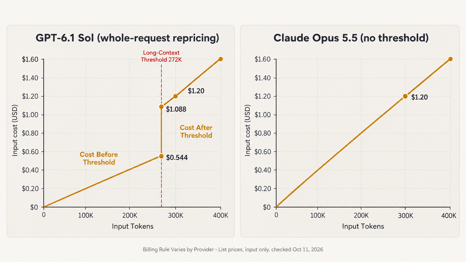
Published 25 October 2026 · Last verified 25 October 2026 · By the UniverseBlend editorial desk On 21 October, Meta set the latest marker for …
agentic AI

What Is Agentic AI? How AI Agents Work, What They Cost, and Where They Fail

Agentic AI describes software systems in which a language model chooses and carries out a sequence of actions to complete a task. It calls tools, …