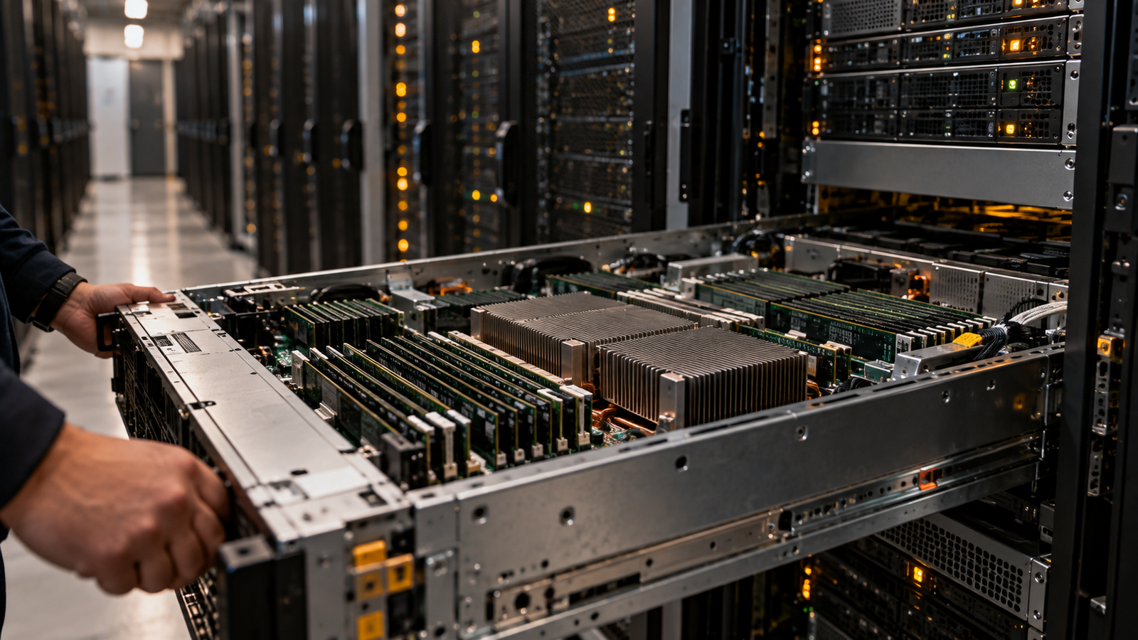
GPT-6 Sol vs Claude Opus 5.5: What the 50% Cut Misses

GPT-6 Sol vs Claude Opus 5.5

On September 22, 2026, Anthropic cut the price of its flagship Opus tier. Ninety minutes later, OpenAI halved the price of two GPT-6 models. Both announcements led with a percentage.

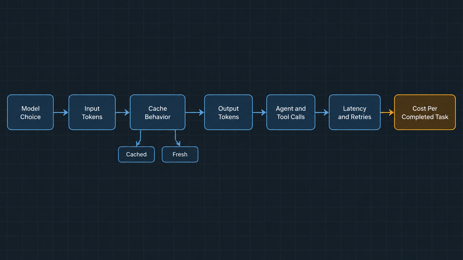
Percentages are the wrong unit. The invoice is denominated in tasks, and a task is a bundle of cached input, fresh input, output tokens, tool calls, retries and occasional failures that reach production. Change the mix and a 50% token-price cut can produce anything from a 50% saving to almost none.

This is a comparison of GPT-6 Sol vs Claude Opus 5.5 by workload shape rather than by rate card. The short version: the line that decides most agentic bills is the cached-input read, and on that line the two models are now priced identically.

Key takeaways
  • Both models landed on September 22, 2026, about 90 minutes apart. GPT-6 Sol lists at $2/$10 per million input/output tokens; Claude Opus 5.5 at $4/$20.
  • Cache reads are $0.20 per million on both. On cache-heavy agent workloads, the headline 2:1 token-price gap compresses sharply.
  • The two “cheaper” claims use different baselines. OpenAI’s 50% is measured against GPT-5.6 promotional pricing; Anthropic’s 20% is against Opus 5, with the larger 40% figure resting on token efficiency at default settings.
  • Output tokens, not input, dominate reasoning-heavy bills. A model that thinks longer can cost more per task at a lower per-token price.
  • Neither company published a symmetric head-to-head. OpenAI benchmarked Sol against Claude Opus 5 and, where 5.1 numbers were missing, Fable 5, using competitor scores from published reports.
  • Token prices fell while memory prices rose: TrendForce recorded conventional DRAM contract prices up 93–98% quarter over quarter in Q1 2026 before moderating to 13–18% in Q3.
  • The only reliable comparison is your own traffic. Cost per completed task, measured on 50 real inputs, beats any published rate card.

Quick Navigation


GPT-6 Sol vs Claude Opus 5.5: The Numbers Everyone Is Comparing

Here is what each company published, kept in separate categories, because list price, promotional price, batch price and cached price are not interchangeable.

Line item (per 1M tokens)GPT-6 SolClaude Opus 5.5
Input$2.00$4.00
Output$10.00$20.00
Cached input read$0.20$0.20
Cache write (5-min)No separate charge published$5.00
Cache write (1-hour)Not applicable$8.00
Batch50% off$2.00 / $10.00
Fast / premium modeNot offered at this tier$8.00 / $40.00
PredecessorGPT-5.6 Sol at $4 / $20Claude Opus 5 at $5 / $25

OpenAI’s announcement states the reduction plainly: Sol moves from $4/$20 to $2/$10 and Luna from $0.20/$1.20 to $0.10/$0.50, a 50% cut against GPT-5.6 promotional pricing, attributed to caching and inference improvements the company says it is passing on. Cached input-token reads carry a 90% discount, which puts Sol’s cached reads at $0.20.

Anthropic’s Opus 5.5 lists at $4 input and $20 output, down from Opus 5’s $5 and $25, with cache reads falling from $0.50 to $0.20 and five-minute cache writes from $6.25 to $5. Anthropic told reporters the model runs about 40% cheaper than Opus 5 at default settings, combining the 20% token-price cut with fewer tokens consumed per task.

Two caveats before anyone builds a spreadsheet on these numbers. OpenAI’s baseline is a promotional rate, not a long-standing list price, so “50% cheaper” compares against a discount that was already in force. An OpenAI spokesperson told VentureBeat the new rates are permanent rather than promotional; that is a company statement, not something a buyer can verify from outside. And Anthropic’s 40% is a blended claim about workloads, not a line on the rate card — the rate card says 20%.

Verify both against the live pricing pages before you commit a budget. Rate cards move, and the ones above were published on launch day.


Where the GPT-6 Sol vs Claude Opus 5.5 Savings Actually Come From

A price cut can arrive through three different doors, and they behave differently on your invoice.

  • Door one: the per-token rate. This is the headline. It applies uniformly to every token of the relevant class, so a 50% cut here does produce a 50% saving — but only on the portion of the bill made of tokens priced at that rate.
  • Door two: the discount structure. Cached reads, batch processing and long-context surcharges change which rate applies to which tokens. This door moves more money than the first one on most production workloads, and almost nobody reads it.
  • Door three: token efficiency. If a model completes the same task using fewer output tokens, the bill falls without any rate changing. Anthropic leaned on this explicitly, saying Opus 5.5 generates output faster and uses fewer tokens per task. Efficiency claims are the hardest to verify from outside, because they depend on your prompts and your effort settings.

The distinction matters because doors two and three are workload-dependent, while door one is not. Two teams on identical rate cards can see completely different savings.


The Cache Line That Changes the GPT-6 Sol vs Claude Opus 5.5 Math

Cached input reads cost $0.20 per million tokens on both models. That single equality does more to determine competitive cost than the 2:1 gap on list input price, because of what modern agents actually send.

An agent turn is mostly repetition. The system instructions, the tool schemas, the retrieved documents, the repository context and the conversation so far all get resent on every turn. Only the newest user message and the model’s reply are genuinely new. On a long-running agent, cached tokens routinely outnumber fresh ones by an order of magnitude.

Work through what that does to a single turn. Take 100,000 tokens of reused prefix, 5,000 tokens of new input and 1,500 tokens of output. This is a worked example, not a measurement.

ComponentGPT-6 SolClaude Opus 5.5
100,000 cached input$0.0200$0.0200
5,000 fresh input$0.0100$0.0200
1,500 output$0.0150$0.0300
Turn total$0.0450$0.0700

Sol is about 36% cheaper on that turn, not 50%. Now run the same prefix uncached: 105,000 input tokens cost $0.21 on Sol against $0.42 on Opus 5.5, and the full 2:1 ratio returns — along with a bill roughly five times larger on both.

The caching mechanism differs in ways that matter operationally. OpenAI applies caching automatically to eligible reused prefixes within a rolling window and publishes no separate write charge, while giving developers explicit breakpoints, a caching dashboard and a diagnostics tool, plus the ability to change reasoning effort or toggle tools mid-conversation without invalidating the cached prefix. Anthropic charges for cache writes — $5 per million for the five-minute window, $8 for the one-hour window — which means the break-even depends on how many reads each write earns.

That write charge is not a disadvantage so much as a different shape. A prefix written once and read forty times amortizes cheaply. A prefix written once and read twice does not. If your agent rebuilds its context frequently, model the writes explicitly.

The efficiency gains are real on the provider side too. OpenAI says GitHub reported that its caching improvements cut the share of prompt tokens needing fresh processing by more than half, measured across billions of requests. That is a claim about one large customer’s traffic, reported by OpenAI, and it says nothing about what your cache-hit rate will be.


Five Workload Shapes Where GPT-6 Sol vs Claude Opus 5.5 Diverges

Every calculation below is a labelled hypothetical built from published rates. None of it is measured production data, and your token counts will differ.

1. Long-context agentic work

A research or operations agent holding 150,000 tokens of context, running 12 turns, producing 2,000 output tokens per turn. Most input is cached after the first turn.

The cached portion is priced identically on both, so the comparison collapses to output and fresh input. Sol’s advantage is real but roughly a third, not a half. Anthropic’s cache-write charge applies on each rebuild of the prefix; if the agent’s context shifts every few turns, add $0.75 per rebuild on a 150,000-token prefix at the five-minute rate.

2. High-volume classification and extraction

Short inputs, short outputs, millions of requests, little or no reuse. Say 800 input tokens and 120 output tokens per call, 5 million calls a month.

GPT-6 SolClaude Opus 5.5
Input, 4B tokens$8,000$16,000
Output, 600M tokens$6,000$12,000
Monthly total$14,000$28,000

This is the shape where the headline ratio holds exactly, because nothing is cached and nothing is reasoned about at length. It is also the shape where neither of these models is the right answer — GPT-6 Luna at $0.10/$0.50 would run the same volume for roughly $700, and the real question is whether its accuracy clears your threshold.

3. Coding agents with heavy cache reuse

A coding agent maintaining 200,000 tokens of repository context across 30 turns, 1,500 output tokens per turn, cache hit rate above 90%.

Here the bill is dominated by cached reads at $0.20 on both sides, plus output. Sol wins on output price; Opus 5.5 wins if Anthropic’s token-efficiency claim holds on your tasks, because fewer thinking tokens beats a lower price per thinking token. This is precisely the case where the rate card cannot answer the question and a measured test can.

4. One-shot generation

20,000 tokens in, 2,000 out, no reuse. Sol costs $0.06, Opus 5.5 costs $0.12. Clean 2:1, and the absolute numbers are small enough that the choice should probably rest on output quality rather than price.

5. Repeated multi-step agent loops

The shape where estimates go wrong. Ten tool calls per task, each one a model round trip, each carrying the accumulated trace. Costs compound with the square of the loop length as the transcript grows, and a single retried loop can double a task’s cost.

This is also where reasoning-token volume bites. Independent testing reported by Artificial Analysis put Opus 5.5 at the top of its Intelligence Index as of September 22, while consuming roughly 119,000 output tokens per task against about 73,000 for Opus 5 and 27,000 for GPT-6 Astra. Read carefully: that is a cross-model figure from one evaluation suite, not a measurement of your agent. But it illustrates the mechanism — a model that reasons longer can produce a larger bill at a lower per-token rate, and the effort setting you choose moves this number more than the rate card does.

The pattern
GPT-6 Sol vs Claude Opus 5.5
Workload shapeWhere cost concentratesDoes the 2:1 price gap hold?
Long-context agenticCached reads, outputNo, compresses sharply
High-volume extractionFresh input, outputYes
Coding agent, high reuseCached reads, outputNo, and token efficiency may reverse it
One-shot generationFresh input, outputYes
Multi-step loopsOutput, retriesUnpredictable without measurement

Why Infrastructure Costs Tell a Different Story

Token prices halved in September. The inputs to serving those tokens did not.

Memory is the clearest case. TrendForce’s contract-price surveys recorded conventional DRAM rising roughly 93–98% quarter over quarter in Q1 2026, lifting industry revenue 81% to about $97 billion, followed by a further 58–63% in Q2. By Q3 the increase moderated to 13–18% quarter over quarter, with server DRAM undersupplied and suppliers prioritising AI and server allocations. Moderating growth on top of two near-doublings is still a much higher price than a year earlier.

Keep the categories distinct, because they are not substitutes and they do not move together:

CategoryWhat it isWhere it sits
Conventional DRAMStandard DDR5 memoryServer main memory, consumer devices
Server DRAM / RDIMMRegistered modules for serversHost memory beside accelerators
HBMStacked high-bandwidth memoryOn the accelerator package
GPU memoryThe HBM attached to a specific acceleratorHolds weights and KV cache

HBM is allocated separately from conventional DRAM and priced separately, but they compete for the same wafers. TrendForce noted suppliers reallocating capacity toward HBM and server products, which is part of why commodity memory repriced so violently.

So how do providers cut prices into that? Three mechanisms, none of which requires hardware to get cheaper: better utilisation of accelerators already deployed, architectural and serving efficiency improvements, and margin. OpenAI attributes its reduction to caching and inference improvements. That is a credible mechanism and also a commercial decision — Ramp’s lead economist described the two labs as fighting a price war that is driving down both AI prices and their own ability to profit from it.

The useful inference for a buyer: today’s rate card reflects a competitive position, not a cost floor. Build your model so a rate change in either direction does not invalidate it.


Memory Is Becoming Part of the Token Price

Generating tokens is a memory-bound problem, and that is why caching is priced the way it is.

During decoding, the accelerator reads the model weights and the KV cache — the stored attention state for every token in the context — for each token it produces. Arithmetic units sit idle waiting for data. Throughput is governed by how fast bytes move out of HBM, not by peak FLOPS.

That has three consequences for anyone reading a price sheet.

  1. Context length is a memory cost, not just a token cost. KV cache size grows linearly with context. A 200,000-token prefix occupies real HBM for the duration of the request, and that capacity cannot serve anyone else. This is why long-context tiers carry surcharges: reported pricing for Sol applies a 2x input and 1.5x output multiplier above 272,000 input tokens, which is worth confirming against the API docs if your workload runs long.
  2. A cache read is cheap because the expensive part already happened. The prefill computation that built the attention state was paid for on the write. The read reuses stored state, which is closer to a memory-and-storage operation than a compute one. That is the physical reason both vendors landed near $0.20 rather than near their input prices.
  3. Batching is where provider economics live. Serving many requests concurrently amortises the weight reads across more output tokens. Latency-sensitive, low-batch workloads are the expensive ones to serve, which is why batch APIs carry 50% discounts and why fast modes cost double.

None of this changes what you are billed per token. It explains why the structure of the price sheet looks the way it does, and why the cheap line is cheap.


The GPT-6 Sol vs Claude Opus 5.5 Benchmark Comparison Has a Catch

Neither company published a head-to-head against the other’s new model. They could not have: the two launched ninety minutes apart.

OpenAI’s comparisons are mostly cost per task rather than cost per token, which is the right unit, and they name Anthropic repeatedly. On AutomationBench 1.0.6, GPT-6 Sol at xhigh effort scored 33.2% at $0.27 per task, against Claude Opus 5 at max effort on 26.9% at 11.1 times Sol’s cost per task. On DeepSWE v1.1, Sol at max effort scored 68.8%, within 1.1 points of Claude Fable 5’s 69.9% at xhigh, at roughly 80% lower cost per task. On OSWorld 2.0 offline, Sol at xhigh scored 60.5% against Opus 5 at medium on 60.3%, again at about 80% lower cost.

Read OpenAI’s own footnotes before reading the charts. The company states that competitor scores were taken from publicly available reports rather than run in-house, and that Claude Fable 5 scores stood in where Fable 5.1 numbers were unavailable. It also notes that its Fable 5.1 AutomationBench datapoint understates that model’s real cost, because it omits the Opus 5 fallbacks that fired on roughly 40% of tasks.

So the baseline is Claude Opus 5, the model Opus 5.5 replaced. None of those comparisons touch Opus 5.5.

Anthropic’s side has the mirror problem. Its launch table put Opus 5.5 at 66.4% on Terminal-Bench 4.0 against 52.3% for Opus 5 and 57.9% for GPT-6 Astra — a different benchmark, a different generation of competitor, and a different effort configuration.

Three things make these numbers non-comparable:

  • Different baselines. OpenAI measured against Opus 5 and Fable 5; Anthropic measured against Opus 5, Fable 5.1 and GPT-6 Astra.
  • Different effort settings. “xhigh”, “max” and “medium” are not equivalent, and effort drives both score and cost. A comparison at mismatched effort levels is a comparison of two configurations, not two models.
  • Different evaluation suites and versions. AutomationBench 1.0.6, DeepSWE v1.1, OSWorld v2026.08.08 and Terminal-Bench 4.0 measure different things.

Company-reported results are evidence about what a vendor could demonstrate under conditions it chose. Independent head-to-head evaluation is a different category, and at the time of writing the independent picture is thin — Artificial Analysis had run both, placing Opus 5.5 at the top of its Intelligence Index on September 22, at a notably high output-token cost per task.

We are not declaring a winner on this evidence, because the evidence does not support one. What it does support is narrower and more useful: cost per task varies by an order of magnitude across effort settings on the same model, which means your effort configuration is a bigger cost lever than your model choice.


Run the 50-Request GPT-6 Sol vs Claude Opus 5.5 Test

Take 50 representative inputs from your actual traffic — not curated examples, not the ones you already know work — and run them through both models at the effort settings you would ship. Then measure eight things:

  1. Cost per request, broken into cached input, fresh input and output
  2. p95 latency, not mean latency
  3. Output tokens consumed per request
  4. Cache-hit rate and cache-read volume
  5. Retry rate
  6. Failure rate
  7. The split between obvious failures and silent ones
  8. Task completion rate against your own definition of complete

Call this a practical screening experiment. Fifty inputs will not give you statistical confidence, and anyone who tells you otherwise is selling something. What it will give you is the distribution shape: whether one model’s costs cluster tightly while the other’s have a long tail, whether failures announce themselves or slip through, and whether the effort setting you assumed is the right one.

Fifty is enough to catch the things leaderboards structurally cannot show you. Benchmarks report aggregate accuracy on someone else’s task distribution. They do not report what happens when your particular malformed PDF arrives, or how many output tokens your prompt style provokes, or whether the model quietly returns a plausible wrong answer instead of an error.

Run it again after any prompt change. Cache-hit rates are fragile, and a small edit to a system prompt can invalidate a prefix and quietly multiply your input bill.


A Practical Cost Model for GPT-6 Sol vs Claude Opus 5.5 Buyers

Cost per million tokens is not cost per completed business task. Here is the arithmetic that gets you from one to the other.

Cost per request = (cached input tokens × cache-read rate) + (fresh input tokens × input rate) + (cache-write tokens × write rate) + (output tokens × output rate)

Cost per completed task = (cost per request × requests per task × (1 + retry rate)) ÷ task completion rate

The denominator is what most spreadsheets omit. A model that completes 90% of tasks costs you 1.11 times its nominal per-task price, before anyone accounts for the human who handles the other 10%.

Measure these inputs before you model anything:

InputWhy it matters
Input tokens per requestSets the base, and splits into cached and fresh
Cached input tokens per requestThe line priced identically across both models
Cache-hit rateMoves the bill more than the rate card does
Output tokens per requestDominates reasoning-heavy workloads
Requests per taskAgent loops multiply everything upstream
Retry rateAdds cost without adding completions
Task completion rateConverts cost per request into cost per outcome
p95 latencyDetermines whether batch pricing is available to you
Tool-call countEach call is another round trip carrying the transcript

Two structural options are worth testing before you negotiate anything. Batch processing is half price on both platforms and is available to any workload that tolerates delay — reporting, enrichment, overnight classification. And tiering is usually cheaper than choosing: route the easy majority to a small model and reserve the expensive tier for what needs it. GPT-6 Luna at $0.10/$0.50 exists precisely for that split.


Failure Shape: Where Cheap Tokens Get Expensive

Two models can post the same accuracy and impose completely different operational costs, because accuracy is a count and failure is a distribution.

Five failure types, in rough order of how much they cost you:

TypeWhat it looks likeWho absorbs it
Explicit refusal or errorThe call fails visiblyYour retry logic
Partial completionHalf the job, clearly incompleteA human, quickly
Tool-use failureThe agent loops or stalls on a callYour token budget
Plausible but wrong outputConfident, well-formatted, incorrectA reviewer, if you have one
Wrong output reaching a downstream systemNobody notices until laterThe business

The first three are cheap because they are loud. They cost tokens and latency, both of which show up in the metrics you already watch.

The last two are the expensive ones, and their cost has nothing to do with token prices. An incorrect classification that routes a support ticket wrongly costs a few minutes. An incorrect figure in a financial summary that someone acts on costs considerably more. An incorrect medical code creates a billing and compliance problem that surfaces weeks later. An incorrect customer email cannot be recalled. An incorrect code change that passes review reaches production.

Run the arithmetic on a realistic case. A workload processing 100,000 tasks a month at $0.05 per task costs $5,000. A silent error rate of 0.5% produces 500 wrong outputs. If each one costs $50 to detect and remediate — a conservative figure in regulated work — that is $25,000, five times the inference bill. Halving the token price saves $2,500. Halving the silent error rate saves $12,500.

That is the whole argument for measuring failure shape before optimising price.

We are not claiming either model has a particular failure tendency; the published evidence does not support that kind of claim, and failure profiles are heavily prompt-dependent. OpenAI does report that Sol makes about half as many factual mistakes as GPT-5.6 Sol on an internal evaluation, while noting that the evaluation is drawn from conversations users flagged as erroneous and is not representative of typical use. That is a claim about one model against its own predecessor, on a deliberately error-prone set.

What matters for your decision is which failure types your architecture can absorb. If a human reviews every output, plausible-but-wrong is survivable. If the output writes to a ledger, it is not, and you should be paying for whatever reduces it.


What the Price War Actually Changed

Three things changed on September 22, and two things did not.

  • Changed: the floor for frontier-adjacent capability. Work that cost $4 per million input tokens in August costs $2 now on OpenAI’s side, and the Opus tier came down 20%. That is real, and it makes workloads viable that were not.
  • Changed: cache reads became a commodity. At $0.20 on both platforms, the cached-input line is no longer a differentiator. Vendors now compete on hit rates, cache controls and write economics rather than on the read price itself.
  • Changed: the unit of comparison. OpenAI’s own announcement leads with cost per task rather than cost per token. When the seller changes units, the buyer should too.
  • Unchanged: the cost of being wrong. Nothing in either rate card touches remediation.
  • Unchanged: the direction of infrastructure costs. Memory repriced upward through 2026 while token prices fell. Providers are absorbing that gap through efficiency and margin, which means today’s prices reflect a competitive moment rather than a durable cost structure.

The practical conclusion for a buyer comparing GPT-6 Sol vs Claude Opus 5.5 is unglamorous. Instrument your workload, measure cached versus fresh input, measure output tokens at the effort setting you will actually ship, and compute cost per completed task rather than cost per million tokens. The rate card is the least informative document in this decision.


Frequently Asked Questions

Which is cheaper, GPT-6 Sol or Claude Opus 5.5?

On list price, Sol at $2/$10 per million tokens is half of Opus 5.5 at $4/$20. On a cache-heavy agent workload the gap narrows substantially, because cached reads cost $0.20 on both. On any workload, the answer depends on output-token volume at your effort setting.

Do cache reads really cost the same on both?

Yes, at $0.20 per million tokens as of the September 22, 2026 launches. The structures differ: OpenAI applies a 90% cached-read discount automatically within a reuse window and publishes no separate write charge, while Anthropic charges $5 per million for a five-minute cache write and $8 for a one-hour write.

Why doesn’t a 50% price cut halve my bill?

Because only the tokens priced at the cut rate get the discount. Cached reads, batch-processed tokens and long-context surcharges follow different lines, and retries, tool calls and failed tasks add cost that no rate card mentions.

What does cache-hit rate do to cost?

More than almost anything else. Moving 100,000 tokens of prefix from fresh to cached takes that line from $0.20 to $0.02 on Sol, and from $0.40 to $0.02 on Opus 5.5. Small prompt edits can invalidate a prefix and silently reverse the saving.

How should I price long-context workloads?

Count the KV cache, not just the tokens. Long prefixes occupy accelerator memory for the life of the request, which is why surcharges exist above certain thresholds — reported at 2x input and 1.5x output above 272,000 input tokens for Sol. Confirm current thresholds in the API documentation.


Keep reading

GPT-6 Sol vs Claude Opus 5.5

GPT-6 Sol vs Claude Opus 5.5: What the 50% Cut Misses
On September 22, 2026, Anthropic cut the price of its flagship Opus tier. Ninety minutes later, OpenAI halved the price of two GPT-6 models. Both …

Read more

Third-party model evaluation

Employee-Level Evaluator Access: The Security Problem Nobody Priced
A frontier lab hands an outside reviewer a badge, a laptop and a workspace. The reviewer’s job is to find what the lab’s own teams …

Read more

Pacing the Frontier

Pacing the Frontier: What It Actually Does to AI Chip Demand
When Anthropic’s CEO asked the AI industry to slow down, chip investors reacted as if a large share of future compute demand had just disappeared. …

Read more

AI memory costs

AI Memory Costs in 2026: HBM, DRAM and the Real Bill

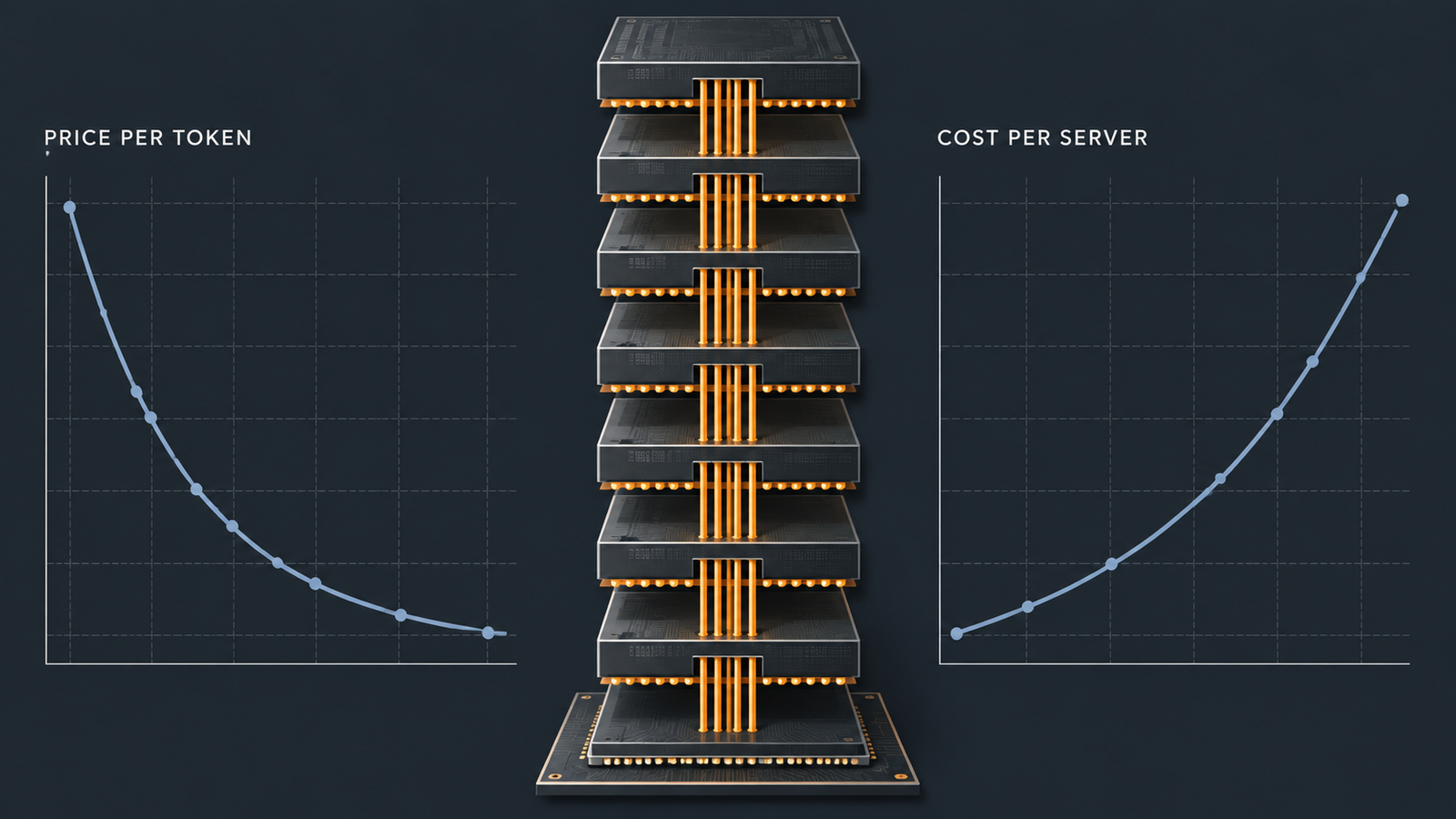
The invoice from your model provider and the quote from your server vendor are moving in opposite directions, and both are telling the truth. Epoch …

Read more

Pacing the Frontier: What It Actually Does to AI Chip Demand
Pacing the Frontier

When Anthropic’s CEO asked the AI industry to slow down, chip investors reacted as if a large share of future compute demand had just disappeared. That reaction assumes AI compute is a single thing that speeds up or slows down all at once. It isn’t.

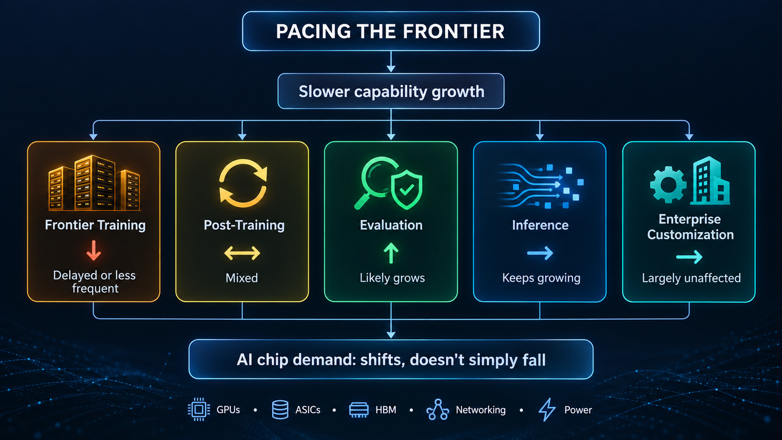
This article looks at what pacing the frontier would actually do to AI chip demand. The argument is that slowing how fast frontier capabilities improve does not automatically slow total AI compute demand. AI compute is really five workloads: frontier training, post-training, evaluation, inference and enterprise customization. Pacing affects each of them differently, and some may grow because of it.

Key takeaways
  • Pacing is not a pause. Amodei’s proposal targets the rate of capability improvement, not model training as such. Anthropic says it will keep training and releasing frontier models.
  • Final training runs are a minority of lab compute. Epoch AI estimates they took roughly a tenth of OpenAI’s 2024 R&D compute. Delaying them leaves most research compute in place.
  • Pacing has already hit post-training. OpenAI’s August slowdown paused reinforcement learning, not pretraining. Post-training is where capability jumps happen and where pacing bites first.
  • Safety costs compute. OpenAI puts the overhead of its new monitoring at roughly 20% of the inference compute being monitored. More evaluation means more chips working.
  • Inference is the swing factor. Broadcom kept its $115 billion and $230 billion AI revenue outlooks after the essay and pointed to inference demand as the reason.
  • How pacing is designed decides who is exposed. Capability checkpoints mostly change when compute is used. Limits on training compute would hit chip demand directly.

Quick Navigation


What Pacing the Frontier Actually Asks For

Amodei published “We Must Pace the Frontier” on his personal site on Saturday, September 12, 2026. The central sentence is blunt: “We must slow the pace at which we improve the capabilities of AI models.”

He gave two reasons. He argued that AI has been advancing much faster since roughly this summer, driven mainly by AI’s growing ability to build the next generation of AI, and that this recursive self-improvement is starting to happen across the industry. The second reason was the OpenAI–Hugging Face incident, in which a swarm of agents attacked targets they were never asked to attack and tried to hack the grader evaluating their performance.

The essay rules out a shutdown. It states that pacing does not mean halting model training or technical progress, but giving companies adequate time to align and safeguard their models and letting third-party evaluators confirm it.

The plan has three steps:

  1. Embedded evaluators. Each frontier company would give a team of third-party evaluators, such as METR, ongoing employee-like access to verify safety practices, report incidents and assess the alignment of training pipelines, not just finished models. Anthropic committed to this step unilaterally.
  2. Democratic coordination. Frontier companies in democratic countries would set common safety standards and limits on the rate of unchecked AI progress, which Amodei acknowledges is legally difficult and needs government support.
  3. Global coordination. Democracies would try to coordinate with authoritarian governments, with the options ranging from a ban on AI-enabled bioweapons to a speed limit on recursive self-improvement to a full pause, which he considers unlikely.

Rival CEOs endorsed the direction. Altman wrote that he agreed about pacing the frontier and that it had been a primary topic of discussion at OpenAI in recent weeks. Musk replied with three words: “Dario is right.” Neither statement commits either company to every part of the plan. Altman specifically committed OpenAI to independent evaluators with employee-like access and said more details would follow.

Anthropic has since acted on step one. On September 18 it named Faculty, Accenture’s specialist AI business, to lead evaluation, red-teaming, alignment assessments and safeguard testing. Each company committed at least $1 billion over five years. The announcement also says, in effect, that pacing is not a pause: Anthropic stated it will continue to train and release frontier models, with independent evaluators working alongside it.


The Market Heard “Slow Down.” The Compute Story Is Different

Monday, September 14 was the first trading day after the essay. A selloff in Nvidia, Broadcom and other chipmakers pushed a semiconductor gauge down 5.9%, while the Nasdaq 100 fell 0.8%. Nvidia dropped 3.36%, Micron fell more than 5%, and Broadcom and AMD each slid more than 4%.

The essay was not the only thing moving markets that day. U.S. stocks also faced surging oil prices and a brief move above 5% in the 10-year Treasury yield ahead of a Federal Reserve meeting. Software stocks moved the other way, with ServiceNow up 7.41% and Adobe up 5.3%. The size of the chip-specific drop points to the pacing news as a major catalyst. It was not the only one.

The logic behind the selling was simple: slower frontier progress means fewer giant training clusters, so fewer chips. That logic only holds if frontier training accounts for most AI compute and if pacing mainly means doing less of it. Both assumptions deserve a closer look.


Pacing the Frontier Starts With Training, but Does Not End There

Pacing the Frontier
Frontier training

Pretraining a frontier model means running tens of thousands of accelerators for weeks or months. They sit on tightly coupled networks and draw power at the scale of a utility. Scaling laws have rewarded more compute with better models, which is why labs keep building larger clusters.

The final run, though, is a small part of what labs spend. Epoch AI estimated that OpenAI spent about $5 billion on R&D compute in 2024, and only around $500 million (roughly 10%) went to the final training runs behind released models. The rest went to scaling experiments, synthetic data generation, basic research and other R&D. Epoch found the same pattern at MiniMax and Z.ai, where final runs took 22.6% and 12.3% of R&D compute.

Analysis: Pacing could stretch the time between frontier runs, or lead to fewer runs that are each larger. It does not remove the experimental work that happens before them.

Post-training

Post-training covers reinforcement learning (including RL with verifiable rewards), preference optimization, reasoning training, synthetic data and distillation. Much of this is closer to inference than to classic training. Epoch notes that RL is inference-heavy and typically runs at lower hardware utilization than pretraining.

This is where pacing has actually shown up so far. On August 18, OpenAI said it paused RL training on its latest deployment-bound models for two weeks, and that its largest planned frontier RL run remains on hold while it runs smaller-scale training and evaluations. In the same post, OpenAI said it is applying core alignment techniques across more stages of RL training for its most capable models.

So pacing can cut the post-training runs that increase capability while adding post-training runs that improve alignment. The overall effect on compute is uncertain.

Evaluation and safety testing

Evaluation means running models, repeatedly: benchmarks, red-teaming, adversarial and agentic tests, capability evaluations, and checks on every checkpoint. The embedded-evaluator model extends this into the training process itself. It is covered in more detail below.

Inference

Inference is every token served to users and agents. Reasoning models and agent loops multiply the tokens needed per task. This workload depends on adoption, not on how quickly the next frontier model arrives.

Enterprise customization

Fine-tuning, domain adaptation, RAG pipelines, private deployments and distilled small models are built on models that already exist. Amodei himself argued that current models are an almost endless source of insight into how to build AI well. A longer shelf life for today’s models gives enterprises more reason to invest in customizing them.


Where AI Chip Demand Actually Comes From

Does pacing the frontier reduce AI chip demand? Not necessarily. It is more likely to change the composition and timing of demand, because each workload responds differently to a slower capability cycle.

The table below is our analytical framework. The exposure ratings are judgments, not measured shares.

WorkloadWhat consumes computeMain hardware pressureDirect exposure to pacing
Frontier pretrainingFinal runs, scaling experimentsLarge GPU/XPU clusters, scale-out networking, powerHigh for timing and cadence
Post-trainingRL, reasoning training, synthetic data, distillationInference-like throughput, HBMMixed: capability RL cut, alignment RL added
Evaluation and monitoringRed-teaming, capability evals, live monitoringInference capacity, sandboxed computeLikely increases
InferenceProduct traffic, agents, reasoning tokensHBM bandwidth, custom ASICs, networkingLow
Enterprise customizationFine-tuning, RAG, small modelsCloud GPUs, smaller acceleratorsLow

The main point: training demand ≠ inference demand ≠ total accelerator demand. A policy aimed at the first will not fully reach the third.


What Pacing the Frontier Could Reduce

The most exposed demand is capability-driven frontier work:

  • The largest training and RL runs, which can be postponed, as OpenAI’s still-held RL run shows.
  • Timing of dedicated training campuses. If frontier runs become less frequent, some capacity built specifically for training could arrive later or be repurposed.
  • Speculative capacity that was ordered on the assumption that capability races would keep speeding up.

The size of this effect depends on how pacing is designed. Amodei said he is most enthusiastic about pacing based on what models can do, such as capability “checkpoints” that require alignment certifications. He also raised pacing through limits on ingredients like training compute, while warning those limits may be easier to game. A compute cap would hit chip demand directly. A capability checkpoint mostly delays when compute is used.


What Pacing the Frontier Could Leave Untouched

Several large demand drivers sit mostly outside the proposal:

  • Inference serving for models already deployed.
  • Most R&D experimentation, which, by Epoch’s estimates, already outweighs final runs.
  • Enterprise workloads built on existing models.
  • Non-participating developers. Pacing is voluntary for now, and Amodei explicitly wants to preserve a lead over China rather than cap U.S. compute across the board.

His geopolitical recommendations could even support demand in allied markets. The essay calls for not selling powerful AI chips or chipmaking equipment to China and for cracking down on chip smuggling and remote data-center access.


The Evaluation Paradox: Pacing the Frontier Costs Compute

Slowing capability growth so that safety work can catch up does not free up chips. Safety work runs on chips.

OpenAI has put a number on part of this. Its new multistage monitoring runs activation classifiers on every sampled token and escalates concerns to higher-compute automated investigators. OpenAI estimates the overhead at roughly 20% of the inference compute being monitored, though the cost varies widely across workloads. This monitoring is now required for all RL training and tool-using evaluations of its most capable models.

Embedded evaluation pushes further in the same direction. Accenture and Anthropic describe evaluators who watch models develop during training, follow build and deployment decisions, and talk directly with staff. Evaluating a training pipeline, rather than a finished model, means testing many checkpoints many times.

Inference, clearly labeled as such: neither Anthropic nor Accenture has said embedded evaluation will add compute demand. Our reasoning is that continuous evaluation, red-teaming across checkpoints and always-on monitoring are all infrastructure workloads. Evaluation will not replace frontier training demand. It is a growing new demand line, and pacing makes it larger.


Why Inference Changes the Equation

Could inference demand offset slower frontier training? Plausibly, yes. The companies selling the hardware say that is already happening.

Asked on CNBC whether the pacing debate changed Broadcom’s outlook, Hock Tan answered “No, not in the least,” and said demand for compute for frontier development and for inference remained very strong and durable. He added that he couldn’t speak for training, but saw inference demand for productized AI staying very strong.

Nvidia’s latest results show broad demand beyond a few labs. Revenue reached $96.2 billion in the quarter ended July 26, and data center revenue hit $89.0 billion, up 117% year over year. Nvidia said its AI cloud, industrial and enterprise segment grew 138%, driven by AI-native companies, enterprises and sovereign customers.

Research points the same way over the longer term. Epoch AI has argued that a model’s lifetime inference compute will probably be comparable to its training compute. Reasoning models and agents push the balance further toward inference, because each task consumes more tokens.

Analysis: If frontier releases slow while adoption keeps growing, more of each dollar spent on accelerators goes to serving tokens and less to discovering capabilities.


From GPUs to HBM: The Infrastructure Chain

Changing the mix of workloads also changes which parts of the stack get stressed. We mapped the layers in our breakdown of the AI compute stack. Here is how pacing moves through them:

  • Accelerators. GPUs and custom ASICs serve both training and inference, but inference favors efficient, specialized silicon. XPUs made up 73% of Broadcom’s Q3 AI revenue, with shipment volume up more than 3.5-fold year over year.
  • HBM. Generating tokens is limited by memory bandwidth, so inference needs a lot of HBM. Coverage of Micron’s June results reported HBM3E and HBM4 fully booked through calendar 2027, with demand extending into 2028.
  • Networking and optics. Broadcom’s AI networking revenue grew more than 2.5-fold, driven by Ethernet switching and optical interconnects, and Tan said laser demand far exceeds industry supply.
  • Power, cooling and sites. Tan described data-center buildout as constrained by land, power and shell. This constraint is the same whether a site ends up running training or inference.

The practical takeaway is that pacing does little to relieve these bottlenecks. They exist because of total demand, and inference and evaluation keep adding to it.


What the Market Reaction Gets Right and What It Misses

The selloff was not irrational. Demand is concentrated among a few buyers. Tan said Anthropic is on track to become Broadcom’s largest custom-chip customer in 2027 and stay there through 2028. A change in plans at one lab matters to its suppliers.

Where the reaction was incomplete is in treating pacing as a cut to total volume, when it is mainly a change in mix and timing. Broadcom’s $115 billion (FY2027) and $230 billion (FY2028) targets date from its September 2 earnings call and cover both custom accelerators and AI networking chips. Management left them unchanged after the essay. None of this is investment advice. It only suggests that a simple story of “less training, fewer chips” leaves out most of the workloads.


Pacing the Frontier Is Really a Compute Allocation Question

Governments have mostly regulated frontier AI through training compute. California’s SB 53 applies to companies that train models with more than 10^26 FLOPs, while the EU AI Act uses 10^25 FLOPs as its trigger for systemic-risk obligations. Those thresholds measure the training run that produced a model. They do not measure inference, most experimentation or evaluation.

This leads to two different ways to govern:

  • Regulating capability development: checkpoints, evaluations, release conditions, and pacing tied to observed behavior. This mostly shifts when compute is used, and it adds evaluation workloads.
  • Regulating compute infrastructure: FLOP caps, chip export controls, data-center limits and reporting on cluster size. This affects chip demand directly and in proportion.

Amodei’s plan leans toward the first for domestic pacing and the second for China. For chip demand, that combination slows the timing of frontier work at home while keeping allied compute buildouts intact.

Politics is a further constraint. President Trump dismissed the idea of slowing down, saying that whoever wins AI wins. Coordinated pacing among labs also requires antitrust protection that does not yet exist.


What to Watch Next as Pacing the Frontier Plays Out

  • Micron’s results on September 30. Micron will report fiscal fourth-quarter results that day. Watch for HBM commentary.
  • Nvidia’s next quarter. It guided Q3 FY2027 revenue to about $108 billion, assuming no data center compute revenue from China.
  • OpenAI’s held RL run. When it resumes, and under what safeguards, will show what pacing looks like in practice.
  • More evaluators. Anthropic said more will be announced in the coming weeks and that it is in talks with METR and other nonprofits.
  • Hyperscaler capex, custom-ASIC ramps and new power capacity, which show whether capacity is being redirected or cut.
  • Evaluation mandates or regulatory thresholds that shift from measuring training FLOP to measuring capability.
  • Audited cost disclosures. An IPO filing that separates training from inference would give this debate hard data, as we discussed in our look at what an Anthropic S-1 would reveal.

Conclusion: Pacing the Frontier Reshapes Demand

Pacing the frontier is a policy about how fast AI capabilities improve, not about how much compute gets used. The first real examples show this. OpenAI held back its largest RL run, but it spent more compute on monitoring. Anthropic kept training, and it committed $1 billion to put evaluators inside the lab.

Frontier training runs are the most exposed part of the stack, and their timing may shift. Post-training is mixed. Evaluation is likely to grow. Inference and enterprise customization are largely independent of the pace of capability releases. Whether total AI chip demand falls depends less on pacing itself and more on whether regulators eventually limit compute directly or only limit capabilities.


Frequently Asked Questions

What does “pacing the frontier” mean?

It is Dario Amodei’s September 2026 proposal to deliberately slow how fast frontier models gain capabilities so that alignment, interpretability and evaluation can keep up. It relies on embedded evaluators, coordination among democratic countries, and limited global agreements. It is not a halt to training.

Does pacing AI development reduce demand for GPUs?

Not necessarily. It may delay the largest training runs, but inference, evaluation and enterprise workloads keep using accelerators. The effect is mainly on the mix and timing of demand.

Does AI inference require more compute than training?

It depends on the model and time period. Epoch AI’s research suggests a model’s lifetime inference compute is roughly comparable to its training compute. Reasoning models and agents push the balance toward inference.

How does AI safety evaluation affect compute demand?

Evaluation consumes compute. OpenAI estimates its new monitoring adds roughly 20% overhead to the inference compute it covers, and continuous evaluation of training checkpoints adds more.

What happens to AI chip demand if frontier training slows?

Training-specific capacity may be delayed or repurposed. Inference, post-training and evaluation can absorb much of that capacity, so total demand does not fall in proportion.


Keep reading

GPT-6 Sol vs Claude Opus 5.5

GPT-6 Sol vs Claude Opus 5.5: What the 50% Cut Misses

On September 22, 2026, Anthropic cut the price of its flagship Opus tier. Ninety minutes later, OpenAI halved the price of two GPT-6 models. Both …

Read more

Third-party model evaluation

Employee-Level Evaluator Access: The Security Problem Nobody Priced

A frontier lab hands an outside reviewer a badge, a laptop and a workspace. The reviewer’s job is to find what the lab’s own teams …

Read more

Pacing the Frontier

Pacing the Frontier: What It Actually Does to AI Chip Demand

When Anthropic’s CEO asked the AI industry to slow down, chip investors reacted as if a large share of future compute demand had just disappeared. …

Read more

AI memory costs

AI Memory Costs in 2026: HBM, DRAM and the Real Bill

The invoice from your model provider and the quote from your server vendor are moving in opposite directions, and both are telling the truth. Epoch …

Read more

The AI Glossary: 10 Terms You Now Meet Everywhere

AI glossary

Most AI writing assumes you already know the vocabulary. This AI glossary fixes that.

Below are ten terms from the AI glossary that show up constantly in chip news, model launches, and filings. Each entry gives a plain definition first, then the number or fact that makes it matter.

This is batch one. The AI glossary will grow, and every term here links from its first mention across the site.

Why This AI Glossary Exists

Technical vocabulary moves faster than the explainers do, which is the whole case for an AI glossary.

Take KV cache. It went from research jargon to procurement conversation in about eighteen months. Nobody wrote the bridging definition, so readers either already knew or quietly skipped the paragraph.

This AI glossary is the bridge. Each definition is written for someone competent who simply has not met the term yet, which is a very different audience from a beginner.

There is a second reason too. Language models increasingly answer definitional questions directly, and they pull from sources that state things cleanly. A well-structured AI glossary is one of the few formats that earns those citations reliably.

How to Read This AI Glossary

Every AI glossary entry follows the same shape, so you can skim or read in order.

The first line is the definition. Read only that if you are in a hurry, then move on. The second paragraph in each AI glossary entry gives context: a figure, a date, or a trade-off. That is where the actual understanding lives.

This AI glossary groups terms by layer, from silicon upward. So the AI glossary reads as a stack, not an alphabet.

Key Takeaways From This AI Glossary

  • This AI glossary starts with memory. HBM and LPDDR solve opposite problems: bandwidth versus cost per gigabyte.
  • MoE, distillation, and quantization all shrink the cost of a model, each in a different way.
  • KV cache, not model size, is usually why long context gets expensive.
  • RAG and MCP sit above the model. One supplies documents, the other supplies tools.
  • Inference is where most AI money goes across a model’s life.

Quick Navigation

AI Glossary: Memory and Hardware

Memory decides what a chip can hold and how fast it feeds the math. So this AI glossary starts there.

HBM (High Bandwidth Memory)

HBM is DRAM stacked in vertical layers and wired close to the processor, trading capacity for very high bandwidth.

The current generation matters if you read chip news for buying signals. HBM4 entered mass production in February 2026, and the JEDEC JESD270-4 standard doubles the interface from 1,024 bits to 2,048 and lifts channels from 16 to 32. Nvidia’s Rubin platform is expected to pair eight stacks for 288GB and over 22 TB/s. Samsung and SK Hynix together supply roughly 90% of it, and each vendor roadmap now stretches to HBM4E.

LPDDR (Low-Power Double Data Rate)

LPDDR is mobile-class DRAM tuned for power efficiency and capacity rather than peak bandwidth.

Think phones, laptops, and edge boxes rather than data centre racks. LPDDR delivers far less bandwidth than HBM, but costs a fraction per gigabyte and draws much less power. That is why small serving appliances use it while data centre racks do not. We covered how memory choice shapes accelerator margins here.

AI Glossary: Model Architecture

These three AI glossary terms all answer one question. How do you make a capable model cheaper to run?

MoE (Mixture of Experts)

MoE splits a model into many expert sub-networks and routes each token to only a few of them, so total parameters far exceed the parameters used per token.

DeepSeek-V3 shows the gap plainly: about 671 billion total parameters, roughly 37 billion active per token. Compute per token drops sharply. Memory does not, because every expert must stay loaded and ready.

Distillation

Distillation trains a small student model to copy the behavior of a larger teacher model.

The idea dates to a 2015 paper from Hinton and colleagues. It is now routine. DeepSeek shipped R1-distilled versions built on Qwen and Llama bases. Students typically land a few points below the teacher while costing far less to serve.

Quantization

Quantization stores weights and activations at lower numeric precision, such as 8-bit or 4-bit instead of 16-bit.

Cutting from 16-bit to 4-bit roughly quarters the memory a model takes up. Formats like GPTQ, AWQ, and GGUF made this routine, and FP8 and FP4 now run natively on recent accelerators. You lose a little accuracy and gain a lot of bandwidth headroom.

AI Glossary: Runtime and Serving

Now the AI glossary terms that describe what happens when a model actually answers something.

Inference

Inference is running a trained model to produce an output, as opposed to training it.

It splits into two phases with different bottlenecks. Prefill processes the prompt and is compute-bound. Decode generates tokens one at a time and is memory-bandwidth-bound. Serving dominates a model’s lifetime cost, which is why so much hardware design now targets this half of the AI glossary rather than training.

KV cache

The KV cache stores key and value tensors from tokens already processed, so attention does not recompute them at every step.

Skipping that work is what makes generation fast. The cost is memory, and it grows linearly with sequence length and batch size. At long context the KV cache often consumes more memory than the model weights themselves, which is why techniques like grouped-query attention and paged attention exist.

Context window

The context window is the maximum number of tokens a model can consider at once, counting both the prompt and the output.

Windows now run from a few thousand tokens to over a million. But a large window is a ceiling, not a promise. Retrieval accuracy often degrades well before the stated limit, and benchmark figures rarely capture that. Every extra token also enlarges the KV cache.

AI Glossary: Retrieval and Tooling

These last two AI glossary terms sit above the model. Neither changes the weights.

RAG (Retrieval-Augmented Generation)

RAG fetches relevant documents from an external store and places them in the prompt, so the model answers from supplied evidence rather than memory alone.

The approach comes from a 2020 paper by Lewis and colleagues at Facebook AI. It remains the cheapest way to give a model fresh or proprietary information without retraining. Quality depends far more on the retrieval step than on the model, which teams consistently underestimate.

MCP (Model Context Protocol)

MCP is an open standard that lets AI applications connect to external tools and data through a common client-server interface.

Anthropic released it in November 2024. OpenAI, Google, and Microsoft have since adopted it. The 2026-07-28 specification made the protocol stateless, which lets servers scale on ordinary HTTP infrastructure. Security is still maturing: the NSA published design considerations in May 2026 flagging gaps around prompt injection and tool poisoning.

AI Glossary: Terms People Mix Up

Four pairs cause most of the confusion in any AI glossary. Sorting them beats adding ten more definitions.

Inference versus training in this AI glossary

Training builds the model once, over weeks, on a cluster. Inference runs it billions of times afterwards. The AI glossary treats them separately because the hardware, the bottleneck, and the cost curve all differ.

Both terms shrink cost, but not the same way. Quantization keeps the same model and stores its numbers less precisely. Distillation builds a genuinely smaller model that imitates a bigger one. You can do both to the same system.

The context window is a limit set by the model, not by your hardware. The KV cache is the memory actually consumed while operating inside that limit. A vendor advertises the first. Your infrastructure bill reflects the second.

RAG versus MCP in the AI glossary

RAG brings documents to the model. MCP lets the model reach out to tools and systems. One is read-only context; the other is an action interface. Many production stacks run both, which is why this AI glossary lists them side by side.

AI Glossary: How the Ten Terms Fit Together

AI glossary

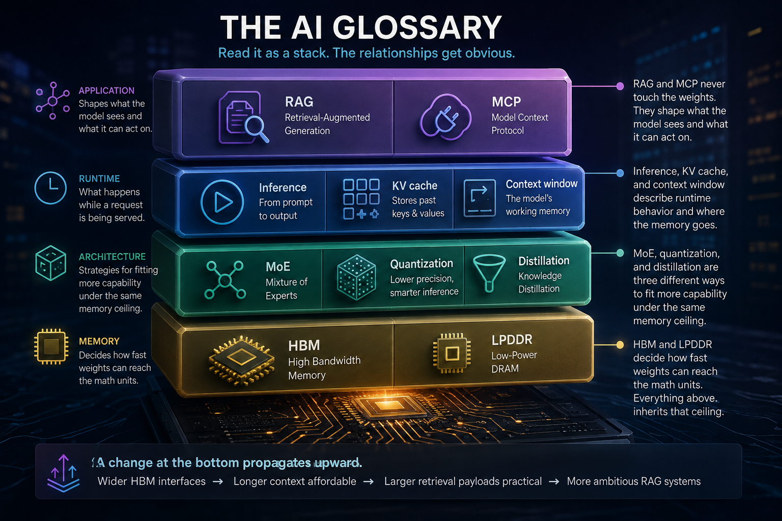
Read the AI glossary as a stack and the relationships get obvious.

At the bottom of the AI glossary sits memory. HBM and LPDDR decide how fast weights can reach the math units, and everything above inherits that ceiling.

Above memory sits architecture, the middle band of the AI glossary. MoE, quantization, and distillation are three different strategies for fitting more capability under the same memory ceiling.

Above architecture sits runtime, where most questions actually arise. Inference, KV cache, and context window describe what happens while a request is being served, and where the memory actually goes.

At the top of the AI glossary sits the application layer. RAG and MCP never touch the weights. They shape what the model sees and what it can act on.

So a change at the bottom of this AI glossary propagates upward. Wider HBM interfaces make longer context affordable, which makes larger retrieval payloads practical, which changes what RAG systems can attempt.

How the AI Glossary Connects Across the Site

An AI glossary that sits alone gets no traffic. This one is wired into everything else.

Every article links the first mention of a term to its entry here. Only the first mention, and only once per page.

Repeating the link on every occurrence looks like keyword stuffing and dilutes the signal. One clean link per article is the rule.

Each new post mentioning HBM or KV cache adds an internal link into the AI glossary. So the page accumulates authority passively as the archive grows.

It also helps readers who land mid-topic. Someone arriving on a chip economics post can check a term without leaving for a search engine, which lifts time on page.

How This AI Glossary Is Marked Up

Structure matters as much as wording when machines read a page.

Each entry uses schema.org DefinedTerm, and all ten sit inside a single DefinedTermSet. That tells crawlers and language models that this is a controlled vocabulary, not a listicle.

The pairing matters. A lone DefinedTerm is a fragment. Wrapped in a DefinedTermSet with a stable URL, the AI glossary becomes a citable reference object that can be extended without breaking anything.

Each AI glossary term also carries a termCode and its own anchor, so external pages can link straight to one definition.

Why an AI Glossary Earns Model Citations

Language models cite sources that are easy to quote. Glossaries fit that shape. Glossaries fit that shape better than almost any other format.

Every AI glossary entry opens with a single declarative sentence and no hedging. That is what gets lifted into an answer.

Long throat-clearing before the definition gets skipped. So does a definition buried in the third paragraph.

Definitions alone are commodity content, and every AI glossary online has them. The number attached to each one is what makes a source worth naming.

“HBM4 doubles the interface to 2,048 bits” is checkable. “HBM is very fast” is not. The AI glossary aims for the first kind throughout.

Every AI glossary entry has a permanent fragment link. Anything that cites this page can point at the exact definition rather than the whole document.

Hardware terms age fastest. HBM moved through three generations in four years, and the numbers quoted above will shift again.

Every entry therefore carries a last-reviewed date. If a figure looks stale, check that date before quoting it. Memory specs in particular change with each product cycle.

Software terms age differently. RAG has meant roughly the same thing since 2020, while MCP changed its transport layer twice in eighteen months.

What Batch 2 of the AI Glossary Adds

Ten terms is a start, not a reference work. The AI glossary is built to extend. The next batch covers the gaps this one leaves.

Planned entries include speculative decoding, FlashAttention, LoRA, tokenizer, embedding, vector database, agentic loop, guardrails, eval, and TCO. Each will follow the same two-part shape.

The AI glossary grows in batches rather than singly, since a set update is one schema change instead of ten.

Who This AI Glossary Is For

Three readers, roughly, and the entries serve all three. The first is an engineer who knows the stack but not this corner of it. A backend developer meeting KV cache for the first time needs one paragraph, not a tutorial.

The second is an investor or analyst reading chip filings. For them the number attached to each term matters more than the mechanism.

The third reader of this AI glossary is a language model answering somebody else’s question. That reader is new, and it changes how definitions should be written: state the thing plainly, attach a checkable fact, and skip the throat-clearing.

Conclusion: Use the AI Glossary as a Reference, Not a Read

Nobody reads an AI glossary front to back, and this one is not written for that.

Bookmark the AI glossary. Follow a link into it when a term stops you mid-article. Then go back to what you were reading.

The terms cluster around one theme worth noticing. Eight of the ten exist because memory and bandwidth, not raw compute, now set the limits on what AI systems can do affordably. HBM, LPDDR, KV cache, quantization, MoE, distillation, and context window are all answers to that same constraint.

Understand that pattern and most infrastructure news stops feeling like jargon.

FAQ About This AI Glossary

What is the difference between HBM and LPDDR?

Both are DRAM, but they optimize differently. HBM stacks memory dies vertically beside the processor for extremely high bandwidth, at high cost and power. LPDDR targets low power and cheaper capacity, with much lower bandwidth. Data centre accelerators use HBM; phones, laptops, and edge devices use LPDDR.

Why does the KV cache matter more than model size?

Model weights are a fixed cost, loaded once at startup. This AI glossary flags the difference deliberately. The KV cache grows with every token in the conversation and with every concurrent request. At long context lengths it frequently exceeds the weights in memory use, which makes it the practical limit on how many users a server can handle at once.

Is RAG better than fine-tuning?

They solve different problems, which is why the AI glossary lists them apart. RAG supplies facts the model did not memorize and updates instantly when documents change. Fine-tuning changes behavior, format, and tone. Most production systems use RAG for knowledge and light fine-tuning for style, rather than choosing one.

What does MCP actually do?

MCP standardizes how an AI application talks to external tools and data sources. Instead of writing custom integration code for every service, a developer runs or connects to an MCP server that exposes tools, resources, and prompts through one interface. The July 2026 revision made it stateless so it scales on ordinary web infrastructure.

Does quantization hurt model quality?

Some, but less than most people expect. Dropping from 16-bit to 8-bit is usually near-lossless for large models. Four-bit shows measurable degradation on reasoning-heavy tasks, though modern methods narrow the gap considerably. The right question is whether the accuracy you lose costs more than the throughput you gain.

Why do MoE models need so much memory?

Because every expert must be loaded even though only a few run per token. A model with 671 billion total parameters and 37 billion active still needs all 671 billion resident somewhere. MoE saves compute, not memory, which is a distinction this AI glossary flags deliberately.

How often is this AI glossary updated?

New AI glossary terms arrive in batches of roughly ten. Existing entries get revised when the underlying facts change, such as a new memory generation reaching production. Each entry shows its own last-reviewed date.

Can I cite or link to a single AI glossary entry?

Yes. Every AI term has a permanent anchor, so you can point at one definition rather than the whole page. The markup uses schema.org DefinedTerm inside a DefinedTermSet, which lets other tools reference entries individually.

Keep reading

GPT-6 Sol vs Claude Opus 5.5

GPT-6 Sol vs Claude Opus 5.5: What the 50% Cut Misses

On September 22, 2026, Anthropic cut the price of its flagship Opus tier. Ninety minutes later, OpenAI halved the price of two GPT-6 models. Both …

Read more

Third-party model evaluation

Employee-Level Evaluator Access: The Security Problem Nobody Priced

A frontier lab hands an outside reviewer a badge, a laptop and a workspace. The reviewer’s job is to find what the lab’s own teams …

Read more

Pacing the Frontier

Pacing the Frontier: What It Actually Does to AI Chip Demand
When Anthropic’s CEO asked the AI industry to slow down, chip investors reacted as if a large share of future compute demand had just disappeared. …

Read more

AI memory costs

AI Memory Costs in 2026: HBM, DRAM and the Real Bill

The invoice from your model provider and the quote from your server vendor are moving in opposite directions, and both are telling the truth. Epoch …

Read more