Generative AI Architecture: The 7 Layers That Are Hard to Undo

generative AI architecture

Published 30 October 2026. API prices checked 28–30 October 2026 on each provider’s official pricing page. Cost figures below are labelled as illustrative where they rest on assumptions.

Every production generative AI architecture has seven layers, from the model at the centre to the security boundary around it. The model is now the easiest of the seven to replace. The commitments that are hard to undo build up in the layers around it: the data pipeline, the evaluation harness, the compute contracts and the trust boundaries.

Teams still spend most of their architecture time comparing models, which makes sense when models change weekly. In the last ten days of October 2026, Moonshot shipped Kimi K3.1 Pro on the 23rd, OpenAI released GPT-6.1 Terra on the 26th and Google announced Gemini 4 Carbon on the 28th, while Gemini 4 Argon prices double on 1 December. A system designed to swap models absorbs all of that in a configuration change.

Key Takeaways
  • Rank the layers by how hard they are to reverse. The model is usually cheapest to change. Security boundaries and data pipelines are the most expensive to retrofit.
  • Calls per request drive the bill more than price per token. In the illustrative deployment below, going from one to three calls per request triples the model bill.
  • Embeddings are cheap. Retrieval operations aren’t. Re-embedding a 50-million-token corpus costs about $1. A million hosted file-search calls cost $2,500.
  • Self-hosting rarely pays at moderate volume. At about 300 output tokens per second on average, most of a rented GPU node sits idle.
  • Build evaluation before you need it. A regression set is cheap on day one and hard to reconstruct after behaviour has drifted.
  • Identity, permissions and egress are architecture, not prompts. Filtering doesn’t stop prompt injection; least privilege limits what an injected instruction can do.

Quick Navigation


The generative AI architecture at a glance

A request passes through the layers in a fairly fixed order. Security authenticates the caller and limits what it may touch. Orchestration picks the steps, retrieval fetches documents and the context layer assembles the prompt. The model runs on the serving layer’s hardware, looping if tools are involved, while evaluation and observability record every step.
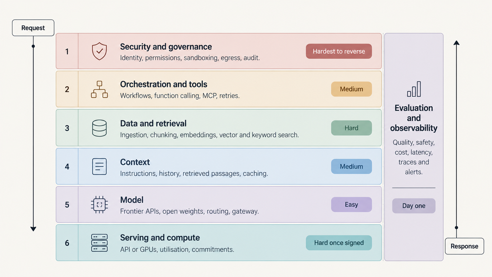
The seven layers of a generative AI architecture

Not every system needs every layer at full strength. A support assistant answering from a product manual might be one model call over a small vector index, with logging, a few hundred regression questions and a server-side API key. An agentic enterprise deployment adds a tool registry, Model Context Protocol (MCP) servers, per-agent identities, sandboxes, egress controls, approval gates and audit retention. Both have seven layers. What changes is how heavy each one is.

The dependencies are uneven. Swapping the model touches context formatting and evaluation. Changing the security model touches identity, tool permissions, network topology and logging, which is nearly everything.

The seven generative AI architecture layers, by cost and reversibility

LayerMain cost driverHow hard to reverseDecide
1. ModelCalls per task × tokens per callEasy, behind a gatewayLate, per task
2. Data and retrievalPipeline engineering, re-indexing, retrieval callsHardEarly
3. ContextRepeated input tokens, cache missesMediumEarly policy, tune later
4. Orchestration and toolsLoop depth, retries, external APIsMediumInterfaces early, frameworks later
5. Serving and computeUtilisation, idle capacity, commitmentsHard once contractedBefore signing
6. Evaluation and observabilityEval runs, judge calls, trace storageCheap early, costly to retrofitDay one
7. Security and governanceIsolation, policy, audit, reviewHardestDay one
Layer 1: the model, the easiest part to replace

The model layer covers frontier APIs, open-weight models you host and the routing logic that sends each task to the right one. A summarisation step doesn’t need the model that writes your migrations. Public leaderboards are a poor guide to that choice, for reasons our piece on why benchmark scores don’t transfer sets out.

Price lists make models look easy to compare. On OpenAI’s pricing page, GPT-6.1 Sol costs $2 per million input tokens, $0.10 cached and $10 output; GPT-6 Luna costs $0.10, $0.01 and $0.50. But the bill depends on how many calls a task needs, how much reasoning the model emits (billed as output) and how often it retries. That’s why cost per completed task is the number to track.

Reversibility depends on a gateway. If every call goes through one internal interface with provider-neutral formats, logging and evaluation, changing models is a config change plus an eval run. If SDK calls are scattered through the codebase, it’s a migration. Decide the gateway early and the model late, and watch the model deprecation tracker, because retirements force switches you didn’t plan.

Layer 2: data and retrieval

Retrieval means ingestion, parsing, chunking, embedding, vector storage, hybrid search, metadata filters and re-ranking, plus the pipelines that keep it current. The embeddings are cheap. OpenAI’s text-embedding-3-small costs $0.02 per million tokens, so embedding a 50-million-token corpus costs about $1. Queries cost more in aggregate: OpenAI’s hosted file search charges $2.50 per 1,000 calls, plus $0.10 per GB per day of storage.

The real cost is reversibility. Chunk size, embedding dimensions, metadata schema and access-control tags end up assumed in prompts, filters, citations and evaluation sets. Change the embedding model and every vector must be regenerated and re-validated against your retrieval tests. Change the chunking and citation offsets break.

Failures here are quiet: stale documents retrieved confidently, permissions leaking because a filter ran after retrieval, a parser dropping the table that held the answer. Decide early how documents carry access rights and versions. Whether you need retrieval at all is covered in RAG versus fine-tuning.

Layer 3: context

Context is everything the model sees on a call: instructions, tool definitions, history, retrieved passages, tool results and memory. A 1M-token window is a ceiling, not a strategy. Every token is billed, delays the first token and can dilute the passages that matter. Context engineering covers what deserves the space.

Prompt caching changes the arithmetic, but only for stable prefixes. Anthropic’s prompt caching charges 1.25 times the input price to write a five-minute cache entry, and cached reads on Opus 5.5 cost $0.20 per million tokens against $4 uncached. Put a timestamp or user ID at the top of the prompt and every call misses.

This layer is medium to reverse: context policies can be rewritten, but answer behaviour and evaluation baselines shift when they are.

Layer 4: orchestration and tools

Orchestration covers prompt templates, workflow engines, function calling, MCP servers, retry policies and agent loops. A system becomes agentic when the model, not your code, decides the next step. That’s where cost becomes variable. A fixed three-step workflow costs three calls. An agent that plans, uses tools and retries might make eight on a good day and twenty on a bad one, each carrying the growing context.

MCP has made tools easier to plug in, and extra agents compound the overhead, as our analysis of multi-agent token cost shows. Individual tools are easy to replace. Workflow state, handoff formats and retry semantics are not, because other components come to depend on them.

Layer 5: serving and compute, where generative AI infrastructure gets committed

The choice is between paying per token and paying per hour, and per-hour only wins when the hardware stays busy. In our GPU cloud pricing survey, checked on 10 October, an 8-GPU H200 node on CoreWeave listed at $50.44 an hour and a single H200 on RunPod at $5.29. The survey’s own example priced H200 output at $0.83 per million tokens at 60% utilisation, which implies roughly 3,000 tokens per second per GPU at full load, or more than 20,000 for the node. The deployment modelled below averages about 300.

That gap is the self-hosting problem. Batching lowers cost per token only when there’s traffic to batch, and peaks, redundancy, engineering time and idle nights all land on your bill, as our breakdown of self-hosted LLM cost shows. APIs bring rate limits instead, but no contract you can’t exit. This layer is easy to change before you sign and hard afterwards.

Layer 6: evaluation and observability

A deterministic service can be tested once. A language model can’t: the same prompt can produce different answers, for reasons covered in LLM determinism. So evaluation means a versioned set of real tasks with pass criteria, run several times per change, with scores reported as ranges. Observability means traces for every model call, tool call and retrieval, tagged with tokens, latency and outcome; our guide to agent observability lists the signals.

The cost is modest early. In the illustrative deployment below, a nightly run of 500 tasks, three attempts each, costs roughly $1,100 a month, and about the same again if an LLM judge grades them (judges have biases, so sample their work by hand). Retrofitting is what gets expensive: without traces from launch, you can’t reproduce last month’s failure or prove a new model isn’t worse.

Layer 7: security, the hardest part of a generative AI architecture to retrofit

Prompt injection is why this layer can’t live in the prompt. OWASP’s LLM01:2025 says “it is unclear if there are fool-proof methods of prevention”, and recommends least privilege, human approval for privileged operations and segregating untrusted content. Filters catch known patterns, but any document or tool result can carry instructions the model follows, across eight distinct injection classes.

What bounds the damage is structural. Each agent gets its own identity, with authorization kept separate from access. Tool permissions are scoped per task. Code runs in isolated sandboxes with egress restricted to named hosts. Secrets stay out of model context, and audit logs attribute every action. NIST’s Generative AI Profile maps the governance actions around this.

None of it is expensive in licences, only in retrofitting. A shared service account baked into ten tools becomes ten migrations.

What a production generative AI architecture costs

This is an illustrative model, not a quote. Token prices are list prices checked on 30 October, GPU prices come from our 10 October survey, and everything else is an assumption.

Assumptions: an internal knowledge assistant handling 1 million requests a month at 1.6 model calls per request, because some requests need a tool and extra calls. Each call sends 8,000 input tokens, including a 3,000-token prefix cached at a 90% hit rate, and returns 500 output tokens, reasoning included. That’s 12.8 billion input and 0.8 billion output tokens a month, about 300 output tokens per second on average.

ScenarioSet-upModel or compute cost per month
A. API-firstEvery call on GPT-6.1 Sol$25,392
A2. API with routing40% of calls on Sol, 60% on GPT-6 Luna$10,932
B. Hybrid40% on Sol; 60% on an open-weight model on two single-H200 pods (redundant), 730 hours each$10,157 + $7,723 = $17,880
C. Primarily self-hostedLarge open-weight model on one 8×H200 node, plus the two pods for small tasks$36,821 + $7,723 = $44,545

Scenario A, per request: 8,480 uncached input tokens at $2, 4,320 cached at $0.10 and 800 output at $10, all per million, come to $0.0254. Across a million requests that’s $25,392. Scenarios B and C exclude the engineering time to run inference, often the largest self-hosting cost.

Retrieval and evaluation sit on top: about $4 a month for query embeddings, $2,500 in hosted file-search fees (a self-managed store avoids those but adds operations work) and roughly $2,300 for evaluation. Three things stand out.

  • Routing beats self-hosting at this volume. Sending the easy 60% of calls to a small API model costs less than renting GPUs for them and keeps capacity elastic, provided the small model passes your evaluation set for those tasks.
  • Self-hosting the large model is the most expensive option here, because a node sized for peaks runs at a tiny fraction of its throughput. At ten or twenty times this volume, with steady traffic, the answer can flip.
  • Calls per request matter most. Holding everything else in scenario A constant, one call per request costs $15,870 a month and three cost $47,610. Losing the cache raises the bill to $33,600; doubling output length raises it to $33,392. A model at half the price that needs twice the calls saves nothing.

Which generative AI architecture decisions to make first

Sort decisions by how much they cost to reverse, not by how urgent they feel.
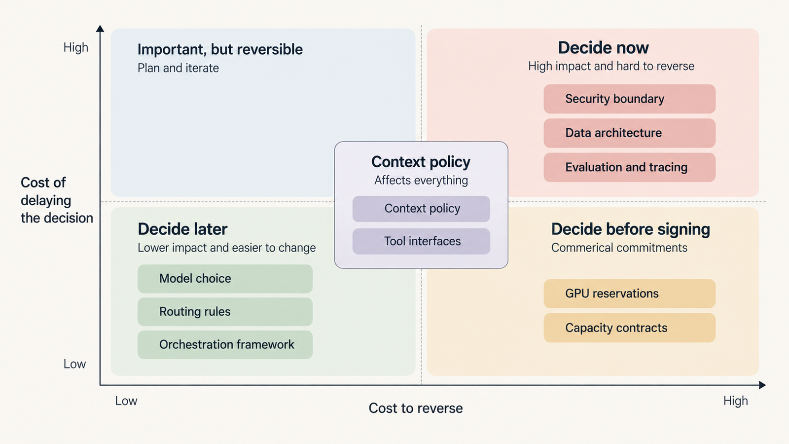
Which generative AI architecture decisions to make first

Decide now: the data architecture (document IDs, versioning, access metadata, re-indexing), the evaluation set and tracing, and the security boundary (agent identity, tool permissions, sandboxing, egress). These shape every other layer.

Decide later: the model, routing rules and most orchestration components. Put them behind interfaces and let evaluation results choose.

Decide before signing anything: reserved capacity and GPU contracts. Wait until real traffic shows sustained utilisation.

A three-person team applies this lightly: one API, a managed vector store, a few hundred evaluation cases and no self-hosting. An enterprise adds weight: a central gateway, data lineage, a shared evaluation service, security review of every tool and procurement rules that block capacity deals without utilisation evidence. The order doesn’t change. The depth does.

A pre-launch generative AI architecture checklist

  • Can you change the model by editing one configuration value and rerunning one evaluation command?
  • Do you know your average and 95th-percentile model calls per request?
  • Is your cache hit rate measured, and is the cached prefix free of per-request values?
  • Can you rebuild the retrieval index from source, and how long does it take?
  • Are access permissions enforced inside the retrieval query?
  • Does every agent have its own identity, with tool permissions scoped to its job?
  • Is outbound traffic from tool execution restricted to an allowlist?
  • Can you replay any production request from its trace?
  • Does a regression set run on every prompt or model change?
  • What is your cost per completed task, and who is alerted when it doubles?
  • If you’ve signed a capacity contract, what was your measured utilisation before signing?

What to remember about generative AI architecture

It’s a set of commitments with different exit costs. The model is the one you’ll change most often, so keep it behind an interface and choose it per task with your own evaluation set. Data pipelines, evaluation and security boundaries outlive several model generations, so design them first. Compute contracts can lock in a cost before you know your traffic, so leave them until utilisation is measured.

Frequently asked questions

What are the seven layers of generative AI architecture?

Model, data and retrieval, context, orchestration and tools, serving and compute, evaluation and observability, and security and governance. They differ most in how hard they are to change later: the model is easiest, security and data hardest.

What is included in a generative AI tech stack?

Typically a model API or self-hosted model, an embedding model and search index, context assembly, an orchestration framework, tool integrations such as MCP servers, an inference platform, evaluation and tracing tools, and identity, secrets, sandboxing and audit infrastructure.

How much does a production generative AI architecture cost?

It depends mostly on calls per request, tokens per call and cache hit rate. In our illustrative example of a million requests a month, model costs ranged from about $11,000 with routing to $25,000 on one frontier API and about $45,000 mostly self-hosted. Engineering and retrieval costs come on top.

What is the difference between API-based and self-hosted inference?

API inference charges per token and scales without capacity planning, but brings rate limits and provider changes. Self-hosted inference charges per GPU-hour whether or not the hardware is busy, so it only wins with sustained high utilisation.

Does every generative AI architecture need a vector database?

No. Small, stable knowledge fits in a cached prompt. Retrieval earns its place when documents are large, change often or need per-user access control, and even then keyword search or a managed store may be enough at first.

Which generative AI architecture components are hardest to change?

Security boundaries and the data architecture, followed by signed compute commitments. Identity, permissions, document metadata and embedding choices spread into every layer. The model is usually easiest, if it sits behind a gateway.


Keep reading

Anthropic IPO valuation

Anthropic IPO: The $895 Billion Question Behind Its Valuation
Last updated: 9 November 2026. Latest confirmed development: Anthropic’s amended S-1, filed on 2 November, still leaves the share count and the IPO price range …
Claude Opus vs Sonnet

Claude Opus vs Sonnet: What the 2026 Price Gap Actually Buys
Last verified: 8 November 2026. All prices are Anthropic’s standard first-party API rates in US dollars per million tokens. They aren’t Claude Pro or Max …
RSA-1024

Did AI Break RSA? What DeepMind Actually Found

Last verified: 8 November 2026. Both papers are unreviewed working papers, and no outside group has reproduced the results yet. No, AI did not break …
Model Distillation

Model Distillation Explained: When AI Learning Becomes Extraction

Last verified: 7 November 2026. Government and company claims are attributed throughout. None has been tested in court. A support team trains a small, cheap …

RAG vs Fine-Tuning: Which One You Actually Need

RAG vs fine-tuning

Take a support team that ships two prototypes on the same base model. The first searches the product documentation on every question and pastes the top passages into the prompt. The second was fine-tuned on 4,000 past tickets. In the demo, the fine-tuned one sounds better: right terminology, exact escalation format. Three weeks later pricing changes. The fine-tuned model keeps quoting the old plan; the retrieval system picks up the new page the morning it’s published.

Neither prototype failed at what it was built to do. Retrieval-augmented generation (RAG) changes what the model can see when it answers. Fine-tuning changes how the model behaves. So the RAG vs fine-tuning decision starts with a plain question: does your problem live in the facts, in the form of the output, or in both?

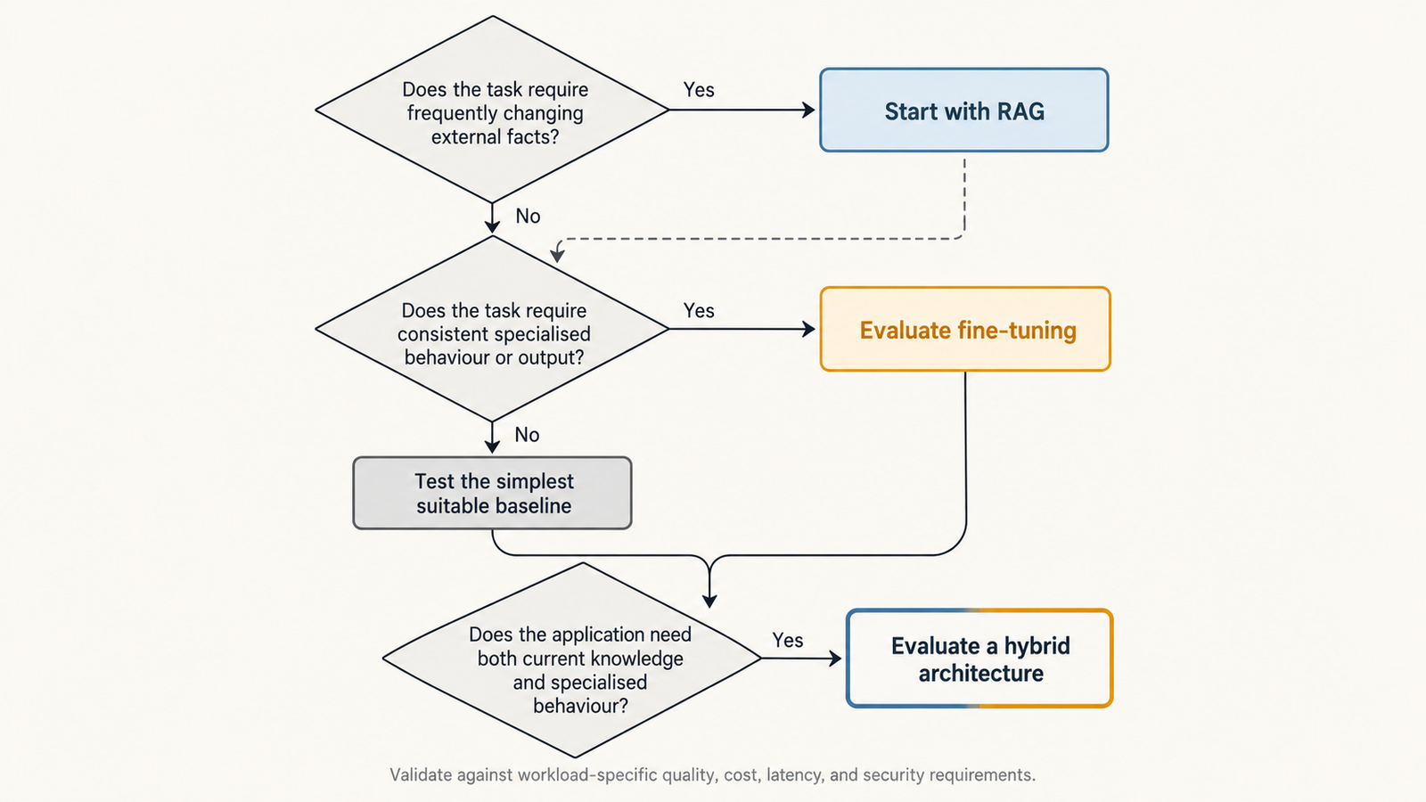
The short answer: start with RAG when answers depend on knowledge that changes, is large, or must be cited. Investigate fine-tuning when the model already knows enough but won’t reliably produce the format, style or task behaviour you need, and prompting hasn’t fixed it. Combine them only when you’ve measured both problems at once.

Key Takeaways
  • RAG updates knowledge at query time without touching weights. Fine-tuning is a weak, risky way to add facts: research found RAG consistently beat it for knowledge injection.
  • Fine-tuning earns its place on behaviour: output format, tone, classification and repeated specialised tasks, especially when it lets you shorten prompts.
  • RAG mostly costs you per query (retrieval plus extra input tokens); fine-tuning mostly costs you per update (data, training, evaluation, regression testing). Query volume and update frequency decide which is cheaper.
  • More retrieved text isn’t better. Models use information in the middle of long contexts less reliably, so retrieval precision beats retrieval volume.
  • Neither approach is a security boundary. Retrieved documents can carry injected instructions; training data can be poisoned.
  • A fine-tuned model is tied to its base model’s lifecycle. On OpenAI’s platform, tuned models are retired along with their base, so budget for re-tuning.

Quick Navigation


RAG vs Fine-Tuning: Two Different Ways to Change an AI System

The original RAG paper by Lewis and colleagues framed the distinction precisely. A model’s weights are parametric memory: knowledge absorbed in training, hard to inspect and hard to update. A searchable document index is non-parametric memory: knowledge the model reads at inference time. The authors pointed to two problems with parametric memory that retrieval helps with, providing provenance for an answer and updating what the model knows.

In a RAG system, the model doesn’t change. At query time the application embeds the question, searches an index, optionally reranks, and inserts the best passages into the prompt. Re-index an edited document and the next answer can reflect it.

Fine-tuning runs a training job on examples of the input and output you want, producing a modified set of weights or a small set of adapter weights. Parameter-efficient methods such as LoRA train a tiny fraction of the parameters (up to 10,000 times fewer than full fine-tuning of GPT-3 175B, the paper reports) without adding inference latency. That makes fine-tuning cheaper. It doesn’t make it a reliable way to store facts.

Five things get lumped together as “teaching the model”:

What needs to changeExampleUsual first tool
KnowledgeCurrent refund policy, a product’s API limitsRAG
BehaviourAsk a clarifying question before actingPrompting, then fine-tuning
StyleHouse tone, terminology, reading levelPrompting, then fine-tuning
Task formatFixed JSON schema, ticket triage labelsStructured outputs or prompting, then fine-tuning
Tool-use patternWhich tool to call, in what orderPrompting and tool definitions, then fine-tuning

Only the first row is about facts. The rest are about form, where fine-tuning has a real case.

RAG vs Fine-Tuning: What Changes When the Source of Truth Changes?

Most enterprise knowledge moves. Product documentation changes each release, policies are revised quarterly, manuals get errata, and support knowledge bases are edited daily. What matters is how often facts change and how quickly a wrong answer hurts.

RAG handles change by re-indexing, but it isn’t instant or automatic. A document edited at 09:00 isn’t retrievable until the ingestion pipeline has chunked, embedded and written it to the index. If the old version isn’t deleted, both can be retrieved and blended. Two sources that disagree, such as a policy page and an outdated FAQ, produce an answer that cites one and contradicts the other. These are data-engineering problems: freshness targets, deletion handling, versioning and source precedence.

Fine-tuning handles change by retraining, and that’s the core reason it’s rarely the first choice for factual knowledge. Ovadia and colleagues compared the two for knowledge injection and found that RAG consistently outperformed unsupervised fine-tuning, for knowledge the model had seen before and for entirely new facts. They also found models struggled to learn new facts this way unless exposed to many variations of each one. A separate study by Gekhman and colleagues found that fine-tuning examples containing new knowledge are learned much more slowly than familiar ones, and that once learned they increase the model’s tendency to hallucinate. Their conclusion: models acquire facts mainly in pre-training, and fine-tuning mostly teaches them to use what they already know.

That doesn’t rule fine-tuning out of fast-changing domains. A claims assistant might retrieve current policy wording while a fine-tuned model handles the stable part: extracting fields into a fixed schema and flagging exceptions consistently. The facts live outside the model; the behaviour lives inside it.

RAG vs Fine-Tuning Cost: The Cost of a Query Versus the Cost of an Update

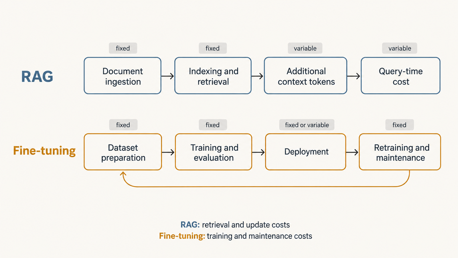
RAG is cheap to change and pays on every query. Fine-tuning pays each time something changes and can be cheaper per query.

  • RAG costs fall into fixed and variable parts. Fixed: preparing documents, building the chunking and embedding pipeline, search infrastructure and re-indexing. Variable, per query: embedding the question, the search, any reranking and, usually the largest line, the extra input tokens from retrieved passages. Evaluation and monitoring sit on top.
  • Fine-tuning costs are weighted the other way. Fixed: curating training examples, training jobs, experiments, evaluation against a baseline and, on every refresh, retraining, regression testing, versioning and rollback. Variable: inference on the tuned model, which may be priced differently from the base model or need dedicated serving if self-hosted.

One fixed cost is easy to miss: a fine-tune is bound to its base model. OpenAI’s fine-tuning guide, checked on 25 October 2026, says the platform is being wound down and closed to new users; existing customers can train until 6 January 2027, and tuned models last only as long as their base model. Whatever your provider, budget for re-tuning and re-evaluating when the base model retires.

A break-even model

Define, over one evaluation period:

  • Q = number of queries
  • C_R = fixed RAG setup and maintenance cost
  • V_R = average variable RAG cost per query
  • C_F = fixed fine-tuning, evaluation and maintenance cost
  • V_F = average variable cost per query on the fine-tuned model

Then:

Total RAG cost = C_R + Q × V_R

Total fine-tuning cost = C_F + Q × V_F

When fine-tuning has the higher fixed cost (C_F > C_R) and the lower per-query cost (V_F < V_R), the volume at which the two totals are equal is:

Q* = (C_F − C_R) / (V_R − V_F)

Below Q*, RAG is cheaper; above it, fine-tuning is. If V_F isn’t lower than V_R, for instance because a tuned model’s per-token premium outweighs the context saved, fine-tuning never breaks even on cost.

Most of the gap V_R − V_F usually comes from context. If fine-tuning lets you drop T_ctx retrieved tokens from every prompt at an input price of P_in per token, then V_R − V_F is roughly T_ctx × P_in plus the retrieval cost, minus any premium the tuned model charges per token. OpenAI’s optimisation guide makes the same point from the other side: fine-tuning can allow shorter prompts with fewer examples and less context, saving tokens at scale. That saving only exists if the facts you were retrieving can be dropped, which is rarely true for changing knowledge.

Three assumptions limit the model. It’s only valid if both systems meet the same quality, latency, security and availability targets. C_F recurs with every data refresh, so frequent updates multiply it. And it ignores the cost of being wrong. Add an error term, with p as the share of answers that are wrong and K as the average cost of a wrong answer (a refund, an escalation, a compliance review), and each total gains Q × p × K. A cheaper system with a higher error rate can cost more overall. UniverseBlend’s breakdown of what inference actually costs per token covers how request shape, caching and batching change V in practice.

RAG vs fine-tuning

Context Length and Inference Latency in RAG vs Fine-Tuning

Every retrieved passage is input the model must process before it writes the first token. That prefill work grows with prompt length, so retrieval adds to time-to-first-token as well as cost. Generation speed changes less with context length than the wait before it starts.

More context also isn’t more accuracy. Liu and colleagues found that models used relevant information best when it sat at the beginning or end of the input and noticeably worse when it sat in the middle, even for models built for long contexts. Retrieving the top 20 chunks “to be safe” can push the one that matters into exactly that position.

The levers are about precision: chunks sized to the unit of meaning (a policy clause, an API endpoint), a reranker that cuts a wide search to a few passages, and compression of long sources. UniverseBlend’s piece on context engineering in AI agents covers how ordering and caching stable prompt sections cut cost and latency, which applies directly to RAG prompts.

Fine-tuning doesn’t make context unnecessary. A tuned model still needs today’s facts, the user’s details and any document it’s asked about. What it can remove is scaffolding: long instructions and few-shot examples that taught the format. That saving is real at high volume, and different from dropping retrieved knowledge.

RAG vs Fine-Tuning: Accuracy, Evaluation and Failure Modes

The two architectures fail in recognisably different ways, and a fluent answer can hide either.

RAG fails when retrieval misses the right passage, the index holds stale or wrong documents, chunk boundaries split the sentence that mattered, the reranker drops key evidence, or the model answers beyond what the text supports. The last is hardest to spot, because the answer arrives with citations.

Fine-tuning fails when training examples are inconsistent (the model learns the errors), when it overfits and handles new inputs worse, when it regresses on abilities the base model had, and when teams assume training on a document means the model will recall it. The Gekhman results suggest that assumption can worsen hallucination.

Evaluate both on a representative test set drawn from real queries, not on demo prompts. For RAG, measure retrieval separately from generation: were the right passages retrieved (recall at k), was the set focused, and was the answer faithful to it? The Ragas framework evaluates these dimensions without human labels for every case. For both, measure correctness, task success, latency and cost per query, and rerun a regression suite on every index rebuild or model version.

RAG vs Fine-Tuning: Security and AI Agent Implications

Retrieval puts external text into the model’s context, and the model can’t reliably tell data from instructions. Greshake and colleagues showed attackers could plant prompts in content an application was likely to retrieve and steer its behaviour and tool calls. In an agent, a poisoned wiki page is an attack path.

Fine-tuning carries a different risk: a model trained on poisoned data carries the problem into every answer, and editing a document won’t fix it. The OWASP Top 10 for LLM Applications 2025 lists both, as prompt injection (LLM01) and data and model poisoning (LLM04), alongside vector and embedding weaknesses (LLM08), which covers retrieval stores themselves.

Neither architecture is a security boundary. Fine-tuning doesn’t reliably train away injection, and phrase filters are easy to evade. The controls that hold sit outside the model: permission-aware retrieval so users only retrieve what they’re allowed to read, provenance on every indexed document, access controls on the index, least-privilege tool permissions and confirmation for irreversible actions. UniverseBlend’s analysis of how agent prompt-injection benchmarks score failures explains why passing a benchmark isn’t proof of safety.

The Facts–Form–Frequency Test: A RAG vs Fine-Tuning Decision Framework

The Facts–Form–Frequency test, developed for this article rather than an industry standard, splits each requirement in two and asks how often each part changes.

  • Facts: what the model must know that it doesn’t reliably know now.
  • Form: how the output must look or behave, consistently.
  • Frequency: how often each changes, and how many queries you’ll serve between changes.

The rules: changing facts go to retrieval. Form that prompting can’t hold goes to fine-tuning, once measured. Frequency and volume decide whether the fixed cost pays.

ScenarioRecommendationAssumption behind it
Frequently changing factual knowledgeRAGUpdates must appear within hours, not training cycles
Stable domain-specific output formatFine-tuning, after prompting and structured outputs fall shortThe format is consistent and examples are available
Repeated specialised task behaviourFine-tuningHigh volume, stable task, measurable gain over prompting
Large collections of reference documentsRAGCorpus too large for the context window and changing
Strict source attributionRAGAnswers must cite the passage they used
High-volume, predictable queriesEvaluate fine-tuning on costQ exceeds Q* at equal quality
Current facts and consistent behaviourBothBoth gaps measured separately
Base model already meets the barNeitherPrompting plus evals pass
RAG vs fine-tuning

When a Hybrid RAG and Fine-Tuning Architecture Makes Sense

A hybrid uses each method for what it’s good at. A fine-tuned extraction model returns contracts in a fixed schema while retrieval supplies the current clause library to check them against.

Hybrids cost more than either alone: you pay C_R and C_F, and a regression could come from the index or the model. Justify one with two measurements, a behaviour gap prompting didn’t close and a knowledge gap the tuned model alone didn’t close. Otherwise start with the simplest architecture that meets requirements, usually a strong base model with good prompting and retrieval.

RAG vs Fine-Tuning: A Workload-Based Implementation Checklist

A planning meeting should be able to answer these before committing:

  1. Baseline: What does the base model score on your test set with good prompting alone?
  2. Test data: Do you have a few hundred real, labelled queries, including hard and adversarial ones?
  3. Update frequency: How often do the underlying facts change, and how stale may an answer be?
  4. Volume: What’s Q per month now and in a year, and what are C and V for each option?
  5. Cost: Are you logging input tokens, retrieval calls and cost per successful task?
  6. Latency: What time-to-first-token and end-to-end targets must hold at peak?
  7. Security: Who may retrieve which documents, which tools can the model call, and what needs human confirmation?
  8. Rollback: Can you revert an index build or model version in minutes?
  9. Lifecycle: When does your base model retire, and who re-tunes and re-tests on its replacement?
  10. Monitoring: Which drop in recall, faithfulness, task success or cost triggers review?

Conclusion

Start with RAG when answers depend on changing facts, a large corpus or a citation requirement. Investigate fine-tuning when the base model knows enough but won’t hold a format, style or task behaviour at your volume after proper prompting. Use both only when you’ve measured both gaps.

The useful next step is small: take 200 real queries, run them through the base model with good prompting, and label every failure as a facts problem or a form problem. The split tells you which approach to build first.

FAQ

Is RAG better than fine-tuning?

Neither in general. RAG suits current or large bodies of knowledge; fine-tuning suits consistent behaviour and format.

Can RAG and fine-tuning be used together?

Yes: a fine-tuned model for task format plus retrieval for current facts. It’s worth the extra cost only when both gaps are measured.

Is RAG cheaper than fine-tuning?

Not always. RAG has lower fixed costs but adds cost to every query; fine-tuning can win at high volume if it removes context, but every update adds fixed cost.

Does fine-tuning add new knowledge to an LLM?

Unreliably. Models learn new facts slowly this way, and learning them can increase hallucination.

Does RAG increase token usage?

Yes. Retrieved passages are extra input tokens on every query. Tighter retrieval and reranking reduce the increase.

Which approach is better for frequently changing information?

RAG. Updating an index takes minutes to hours; updating weights takes a training cycle plus evaluation.

Can fine-tuning improve structured output?

Often. Try structured-output features and prompting first, then fine-tune if format errors persist at your volume.

Does RAG make an AI agent more secure?

No. Retrieved documents can carry prompt injections. Security comes from permissions, provenance and tool controls outside the model.


Keep reading

Anthropic IPO valuation

Anthropic IPO: The $895 Billion Question Behind Its Valuation

Last updated: 9 November 2026. Latest confirmed development: Anthropic’s amended S-1, filed on 2 November, still leaves the share count and the IPO price range …
Claude Opus vs Sonnet

Claude Opus vs Sonnet: What the 2026 Price Gap Actually Buys

Last verified: 8 November 2026. All prices are Anthropic’s standard first-party API rates in US dollars per million tokens. They aren’t Claude Pro or Max …
RSA-1024

Did AI Break RSA? What DeepMind Actually Found

Last verified: 8 November 2026. Both papers are unreviewed working papers, and no outside group has reproduced the results yet. No, AI did not break …
Model Distillation

Model Distillation Explained: When AI Learning Becomes Extraction

Last verified: 7 November 2026. Government and company claims are attributed throughout. None has been tested in court. A support team trains a small, cheap …

LLM Context Window Comparison 2026: Limits and Costs

LLM context window

Specifications and prices checked October 11, 2026 · Prices in USD per million tokens, standard API tier

Short answer: In an LLM context window comparison for 2026, input capacity barely separates the leading models. Every proprietary API checked here accepts about 1 million tokens (1M to 1,050,000), and the two open-weight hosts list 1M or 524,288. Output caps differ more, from 65,536 tokens on Gemini to 128,000 on GPT-6.1 Sol and Claude Opus 5.5. Long-context pricing rules differ most of all: a 300,000-token prompt costs anywhere from $0.06 to $1.20 in input charges.

Three numbers get conflated in most spec sheets. The context window is how much a model can read in one request. The output limit is how much it can write back. The long-context pricing threshold is the prompt size at which the provider starts charging more. A model can have a huge window, a modest output cap and a threshold that doubles your bill well before you get near the window’s edge.

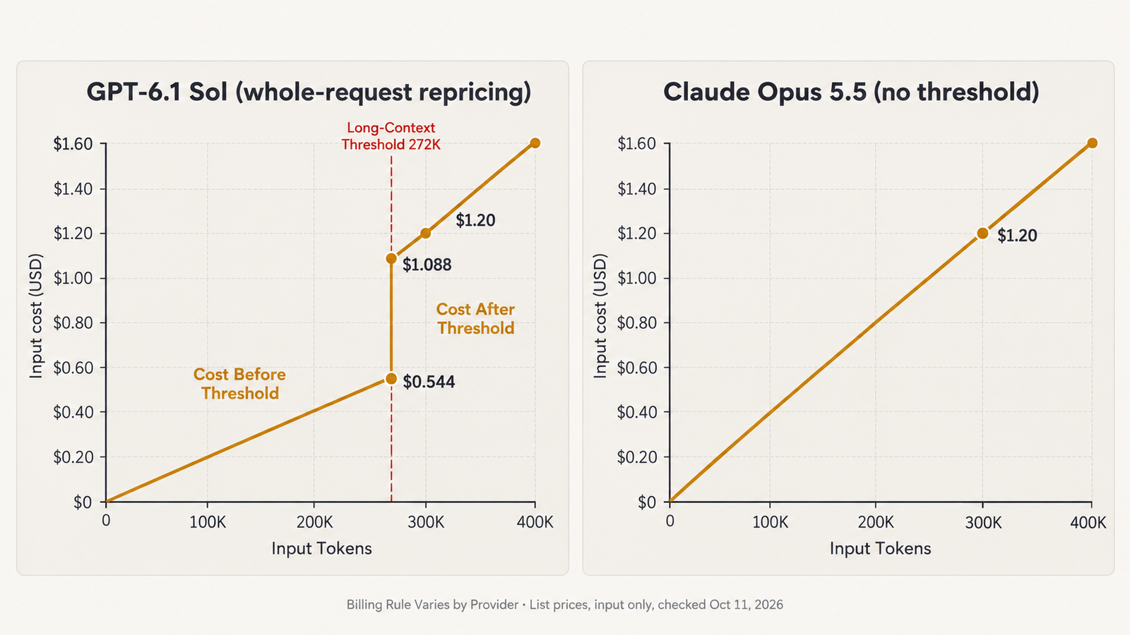
The third number is the one buyers skip. GPT-6.1 Sol charges $2.00 per million input tokens up to 272,000 tokens and $4.00 per million above it, and OpenAI applies the higher rate to the full request. A 270,000-token prompt costs $0.54. A 280,000-token prompt costs $1.12. Ten thousand extra tokens cost 58 cents.

Key Takeaways
  • Context capacity has converged. Every proprietary model checked lists about 1M input tokens, so window size rarely decides a purchase in 2026.
  • Output caps have not converged. Gemini 3.1 Pro and 3.8 Flash cap output at 65,536 tokens, about half of GPT-6.1 Sol’s and Claude Opus 5.5’s 128,000.
  • Three providers reprice by prompt size. OpenAI does it above 272K for the whole request, Google above 200K for Gemini 3.1 Pro, and Anthropic above 100K for Claude Haiku 5.5 only.
  • Claude Opus 5.5 and Sonnet 5.5 have no long-context surcharge. At 300K tokens, Opus 5.5 ($1.20) costs the same as GPT-6.1 Sol and Gemini 3.1 Pro, even though its base rate is twice theirs.
  • Crossing a threshold can cost more than the extra tokens are worth. Just past 272K, a GPT-6.1 Sol prompt more than doubles in price.
  • Caching flattens the comparison. A fully cached 300K prefix costs $0.06 on both GPT-6.1 Sol and Claude Opus 5.5.
  • Open-weight hosting is cheapest per token, but a host’s served context can differ from the model card. Check the endpoint, not the paper.

Quick Navigation


The LLM context window comparison table

All values are taken from official documentation and were checked October 11, 2026. “Threshold” is the prompt size at which input pricing changes. Costs cover input tokens only, with no output, caching, batch discounts or taxes.

Model and versionMax input contextMax outputLong-context thresholdInput belowInput above300K input costAvailabilityDocumentation
GPT-6.1 Sol (gpt-6.1-sol)1,050,000128,000>272K, whole request$2.00$4.00$1.20GA, OpenAI APIModel page
GPT-6 Luna (gpt-6-luna)1,050,000128,000>272K, whole request$0.10$0.20$0.06GA, OpenAI APIModel page
Claude Opus 5.5 (claude-opus-5-5)1M128,000None$4.00n/a$1.20Current, Claude APIModels · Pricing
Claude Sonnet 5.5 (claude-sonnet-5-5)1M128,000None$2.00n/a$0.60CurrentSame as above
Claude Haiku 5.5 (claude-haiku-5-5)1M128,000>100,000$0.10$0.50$0.15CurrentSame as above
Gemini 3.1 Pro (gemini-3.1-pro-preview)1,048,57665,536>200K$2.00$4.00$1.20PreviewModel · Pricing
Gemini 3.8 Flash (gemini-3.8-flash)1,048,57665,536None$0.75 (to Dec 31, 2026; $1.50 from Jan 1, 2027)n/a$0.225StableModel
Gemini 3.5 Flash-Lite (gemini-3.5-flash-lite)1,048,57665,536None$0.30n/a$0.09StableModel
Mistral Large 4 (mistral-large-4)1MNot publicly documentedNone documented$0.68 sale ($1.36 list)n/a$0.204 salePublic Preview, open-weightModel page
Llama 4 Maverick (Together AI)1M per model card; host lists 1,048K and 524,288Not publicly documentedNone documented$0.27n/a$0.081Hosted endpointModel card · Host
Qwen3.8-2.4T-A95B (Together AI)262,144 native; 1M served131,072None documented$2.00n/a$0.60Hosted endpointModel card · Host

Whole-request rules apply where stated. OpenAI says prompts above 272K are “priced at 2x input and cache rates and 1.5x output for the full request.” Anthropic says a Haiku 5.5 request over 100,000 tokens “pays the higher prices,” counting cache reads and writes toward prompt length. Google’s table selects the rate by prompt size (“prompts > 200k tokens”) but does not explicitly say the whole prompt is repriced. This article assumes it is, and that is an interpretation of Google’s wording.

The open-weight rows describe one host’s endpoint, not the model. Qwen3.8’s model card gives 262,144 tokens natively, extensible to about 1M. A 300K request on Together therefore runs in the extended range, where quality can differ from native-length behaviour.

Context window versus output limit

The context window caps what goes in. The output limit caps what comes out in a single response. They are documented separately for every proprietary model here, and they constrain different workloads.

Output limits bind harder than input limits. A model that reads a 400-page contract can only write 65,536 tokens back if it is Gemini 3.1 Pro, or 128,000 if it is GPT-6.1 Sol or Claude Opus 5.5. That is roughly 50,000 versus 100,000 words, before any reasoning tokens. Google bills thinking as output (“output price including thinking tokens”), so whether reasoning also draws on the output cap matters for long reasoning tasks. Check each provider’s documentation for that point, because accounting differs.

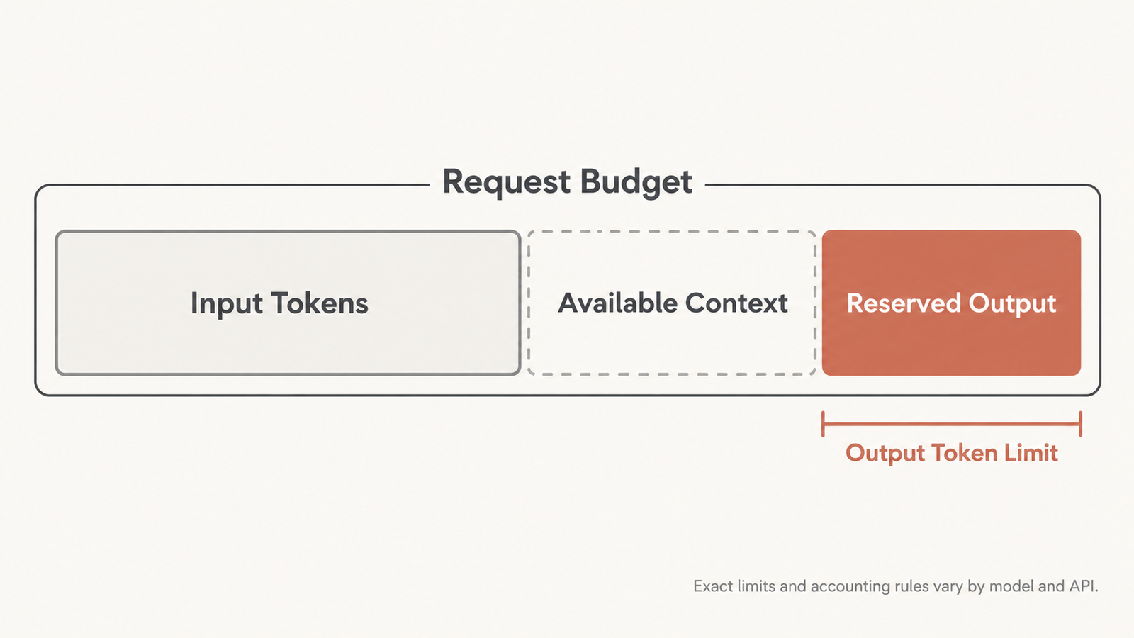
Some providers also treat input and output as one shared budget, so a large prompt leaves less room to answer. Qwen’s model card illustrates the general point: it recommends allowing 262,144 tokens for reasoning and 131,072 for the final answer, figures that only make sense if the request budget is planned as a whole.

LLM context window

Where long-context pricing start

Three of the providers checked charge more once a prompt gets long. Each draws the line in a different place and handles it a little differently.

  • OpenAI, 272K, whole request. For GPT-6.1 Sol and GPT-6 Luna, prompts above 272K input tokens pay double the input and cache rates and 1.5 times the output rate, on every token in the request. OpenAI’s pricing page lists the long-context column, and the threshold and the “full request” rule appear on each model page.
  • Google, 200K, by prompt size. Gemini 3.1 Pro charges $2.00 input and $12.00 output for “prompts <= 200k tokens”, and $4.00 and $18.00 for larger prompts. Context caching moves from $0.20 to $0.40. Gemini 3.8 Flash and 3.5 Flash-Lite have no split.
  • Anthropic, 100K, Haiku only. Anthropic’s pricing documentation states that its current models other than Claude Haiku 5.5 “include the full 1M token context window at standard pricing”, adding that “a 900k-token request is billed at the same per-token rate as a 9k-token request.” Haiku 5.5 moves from $0.10 to $0.50 per million input tokens above 100,000 prompt tokens, a fivefold jump, and cache reads count toward that total.

Mistral and the two open-weight hosts publish no threshold.

One ambiguity matters for anyone sizing prompts close to a boundary. Neither OpenAI nor Google says whether “272K” or “200K” means thousands or multiples of 1,024 tokens. The calculations below avoid the gap by testing well clear of either reading.

What a 300K-token request costs

The scenario: one request with 300,000 input tokens, zero output and no caching. It isolates the input-side effect of each pricing rule. These are author calculations from the official prices above, in USD.

Formula, where the provider reprices the whole request once a prompt crosses threshold T:

\text{Input cost} = \frac{N}{1{,}000{,}000} \times \begin{cases} r_{\text{standard}} & N \le T \\ r_{\text{long}} & N > T \end{cases}
Just below and just above each threshold
ModelBelow thresholdCostAbove thresholdCostJump
GPT-6.1 Sol270,000 tokens$0.540280,000 tokens$1.120+$0.58 for 10K more tokens
GPT-6 Luna270,000$0.027280,000$0.056+$0.029
Gemini 3.1 Pro190,000$0.380210,000$0.840+$0.46 for 20K more tokens
Claude Haiku 5.599,000$0.0099101,000$0.05055.1x for 2% more tokens
At 300,000 tokens
ModelRate applied300K input cost
GPT-6.1 Sol$4.00 (long-context)$1.20
Claude Opus 5.5$4.00 (standard)$1.20
Gemini 3.1 Pro (preview)$4.00 (long-context, assumed whole prompt)$1.20
Claude Sonnet 5.5$2.00$0.60
Qwen3.8-2.4T-A95B on Together$2.00$0.60
Gemini 3.8 Flash$0.75 (2026 rate)$0.225
Mistral Large 4 (preview)$0.68 sale / $1.36 list$0.204 / $0.408
Claude Haiku 5.5$0.50 (long-context)$0.15
Gemini 3.5 Flash-Lite$0.30$0.09
Llama 4 Maverick on Together$0.27$0.081
GPT-6 Luna$0.20 (long-context)$0.06

The three-way tie at the top is the central finding. On list prices, Claude Opus 5.5 costs twice as much as GPT-6.1 Sol per input token. At 300K tokens, OpenAI’s threshold has already doubled Sol’s rate and Google’s has doubled Gemini 3.1 Pro’s, while Opus stays flat. All three land at $1.20. Below 200K, Opus costs twice as much as either. Above 272K, the gap disappears.

Separate scenario: adding an 8,000-token answer

Keep the 300K prompt and add 8,000 output tokens. OpenAI’s long-context rule raises Sol’s output rate to $15.00 per million, and Google’s raises Gemini 3.1 Pro’s to $18.00.

  • GPT-6.1 Sol: $1.20 + (8,000 / 1M × $15) = $1.32
  • Gemini 3.1 Pro: $1.20 + (8,000 / 1M × $18) = $1.344
  • Claude Opus 5.5: $1.20 + (8,000 / 1M × $20) = $1.36
  • GPT-6.1 Sol at 270,000 input tokens instead: $0.54 + (8,000 / 1M × $10) = $0.62

Trimming 30,000 tokens from the prompt halves Sol’s bill. For Opus, the same trim saves about 9%.

LLM context window

Context window choices for RAG, coding and agents

  1. RAG pipelines. Retrieval systems control their own prompt size, which makes them the easiest place to exploit a threshold. A pipeline that routinely sends 250,000 to 300,000 tokens to GPT-6.1 Sol is paying the long-context rate on a share of requests that a retrieval cap of about 260,000 would remove. On Claude Opus 5.5 there is no such boundary to manage.
  2. Long-document analysis. Reading a large filing and returning a short summary is the case where big windows pay off most cleanly: input-heavy, output-light. The output cap rarely matters here, and the threshold often decides the bill.
  3. Coding agents. Consider an illustrative repository-aware agent that resends 300,000 tokens of code context on every turn. Without caching, 20 turns on GPT-6.1 Sol cost 20 × $1.20 = $24 in input alone. If the repository context is a stable prefix, OpenAI’s long-context cached rate of $0.20 per million drops each turn’s input to $0.06. That is why caching usually changes these comparisons more than the threshold does.
  4. Multi-agent systems. When several agents each carry a copy of a shared history, every copy is billed separately and pushed toward the threshold on its own. Summarising or pruning shared state before handoff can keep each call below a boundary that the combined history would cross.
  5. Long-running agents. Tool results accumulate. An agent that starts at 50,000 tokens and appends 10,000 per step crosses Gemini 3.1 Pro’s 200K line at step 16 and Sol’s 272K line at step 23. From that point every turn is billed at the higher rate. Compaction policies are cost controls, not just memory management.
  6. Prompt caching. Caching narrows the gap between providers on repeated context. At long-context rates, a fully cached 300K prefix costs $0.06 on GPT-6.1 Sol ($0.20 per million) and $0.06 on Claude Opus 5.5 ($0.20 per million cache hit). UniverseBlend’s earlier analysis of why a 50% price cut doesn’t halve agent bills made the same point for shorter contexts: once cache reads dominate, list-price gaps shrink. Note that Anthropic counts cache reads toward Haiku 5.5’s 100K threshold, and OpenAI doubles cache rates above 272K, so caching does not exempt a request from repricing.
  7. Splitting requests. Two 150,000-token GPT-6.1 Sol calls cost $0.60 in input, half the price of one 300,000-token call. That only works if the task decomposes. Cross-document reasoning does not split cleanly, and any shared instructions are paid twice. For Opus 5.5, splitting saves nothing on price.

A usable context budget is smaller than the advertised window. Rate limits measured in tokens per minute fill faster with long prompts, which UniverseBlend covered in AI API rate limits in 2026. This article makes no latency claims, but longer prompts add processing time before the first token.

A context window checklist before you choose

  • Measure your real prompt-size distribution, including p95, not just the average
  • Find each candidate’s threshold and whether it reprices the whole request
  • Check the output cap against your longest required answer, including reasoning tokens
  • Price the workload with your actual cache-hit rate
  • Confirm the hosted endpoint’s served context for open-weight models, not just the model card
  • Note preview status (Gemini 3.1 Pro, Mistral Large 4) and dated price changes (Gemini 3.8 Flash on January 1, 2027)
  • Check tokens-per-minute limits at your prompt size
  • Test quality at your real context length; a model accepting 1M tokens says nothing about how well it uses them

Conclusion

This LLM context window comparison shows the window itself has stopped being a differentiator. Nearly everything accepts about a million tokens. What separates the models is the output cap, whether the model is still in preview, and above all the pricing rule waiting at 100K, 200K or 272K tokens.

For workloads that sit under 200K tokens, list prices are a fair guide. For workloads that regularly cross 272K, a model with no surcharge can match one with half its base rate, and trimming a prompt by 10% can halve the bill. Price your real prompt distribution against each provider’s rule before trusting the headline number.

Frequently Asked Questions

What is the difference between an LLM context window and an output token limit?

The context window is the maximum input a model accepts in one request. The output limit is the maximum it can generate in one response. As of October 2026, most leading models accept about 1M input tokens, but output caps range from 65,536 (Gemini) to 128,000 (GPT-6.1 Sol, Claude Opus 5.5).

Does a larger context window always mean a better model?

No. Capacity says nothing about how well a model uses long context, and the largest windows now look nearly identical across providers. Output limits, pricing thresholds and quality at your real prompt length matter more.

What happens when a request exceeds the context window?

The API generally rejects it or requires you to shorten the input. Exact error behaviour varies by provider. Applications should count tokens before sending and trim, summarise or split oversized inputs.

How does long-context pricing work?

Some providers charge a higher per-token rate once a prompt passes a set size. In October 2026 that meant 272K for OpenAI’s GPT-6.1 Sol and GPT-6 Luna, 200K for Google’s Gemini 3.1 Pro, and 100K for Anthropic’s Claude Haiku 5.5. Claude Opus 5.5 and Sonnet 5.5 have no surcharge.

Does crossing a pricing threshold reprice the entire request?

For OpenAI, yes: the documentation says the higher rates apply “for the full request.” Anthropic’s Haiku 5.5 rule also applies the higher price to any request over the threshold. Google selects the rate by total prompt size but does not state the whole-request rule as explicitly.

Can prompt caching reduce long-context costs?

Yes, often by more than avoiding a threshold. A fully cached 300K prefix costs $0.06 on GPT-6.1 Sol or Claude Opus 5.5, against $1.20 uncached. Caching does not exempt a request from long-context repricing, though.

How should developers compare proprietary and open-weight models?

Compare the specific hosted endpoint, not the model card. A host may serve a different context length than the paper describes. Qwen3.8’s native 262,144-token context is extended to 1M on Together AI, for example.

What should an AI agent developer measure before choosing a model?

Prompt-size growth per step, the step at which each provider’s threshold is crossed, output needs per turn, cache-hit rate and tokens-per-minute limits. Then test answer quality at the context length the agent actually reaches.


Keep reading

Anthropic IPO valuation

Anthropic IPO: The $895 Billion Question Behind Its Valuation

Last updated: 9 November 2026. Latest confirmed development: Anthropic’s amended S-1, filed on 2 November, still leaves the share count and the IPO price range …
Claude Opus vs Sonnet

Claude Opus vs Sonnet: What the 2026 Price Gap Actually Buys

Last verified: 8 November 2026. All prices are Anthropic’s standard first-party API rates in US dollars per million tokens. They aren’t Claude Pro or Max …
RSA-1024

Did AI Break RSA? What DeepMind Actually Found
Last verified: 8 November 2026. Both papers are unreviewed working papers, and no outside group has reproduced the results yet. No, AI did not break …
Model Distillation

Model Distillation Explained: When AI Learning Becomes Extraction

Last verified: 7 November 2026. Government and company claims are attributed throughout. None has been tested in court. A support team trains a small, cheap …

The AI Glossary: 10 Terms You Now Meet Everywhere

AI glossary

Most AI writing assumes you already know the vocabulary. This AI glossary fixes that.

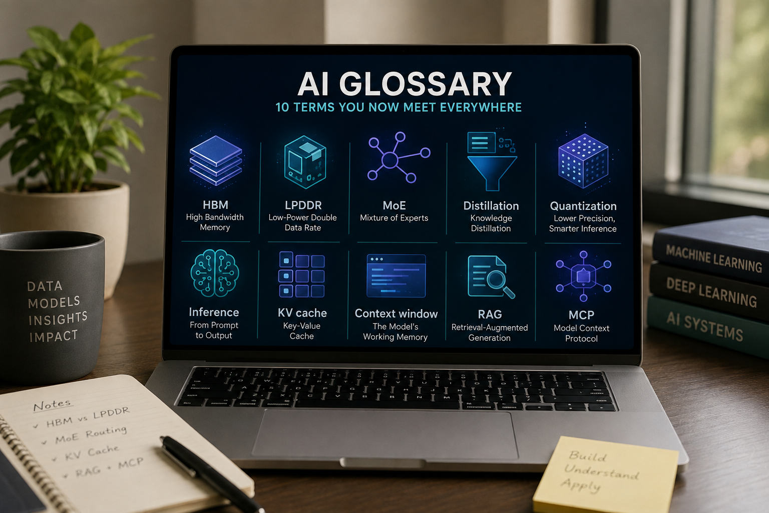
Below are ten terms from the AI glossary that show up constantly in chip news, model launches, and filings. Each entry gives a plain definition first, then the number or fact that makes it matter.

This is batch one. The AI glossary will grow, and every term here links from its first mention across the site.

Why This AI Glossary Exists

Technical vocabulary moves faster than the explainers do, which is the whole case for an AI glossary.

Take KV cache. It went from research jargon to procurement conversation in about eighteen months. Nobody wrote the bridging definition, so readers either already knew or quietly skipped the paragraph.

This AI glossary is the bridge. Each definition is written for someone competent who simply has not met the term yet, which is a very different audience from a beginner.

A glossary also gives readers a stable reference when an article uses unfamiliar terminology. A clear definition and a direct link help readers check the meaning in context.

How to Read This AI Glossary

Every AI glossary entry follows the same shape, so you can skim or read in order.

The first line is the definition. Read only that if you are in a hurry, then move on. The second paragraph in each AI glossary entry gives context: a figure, a date, or a trade-off. That is where the actual understanding lives.

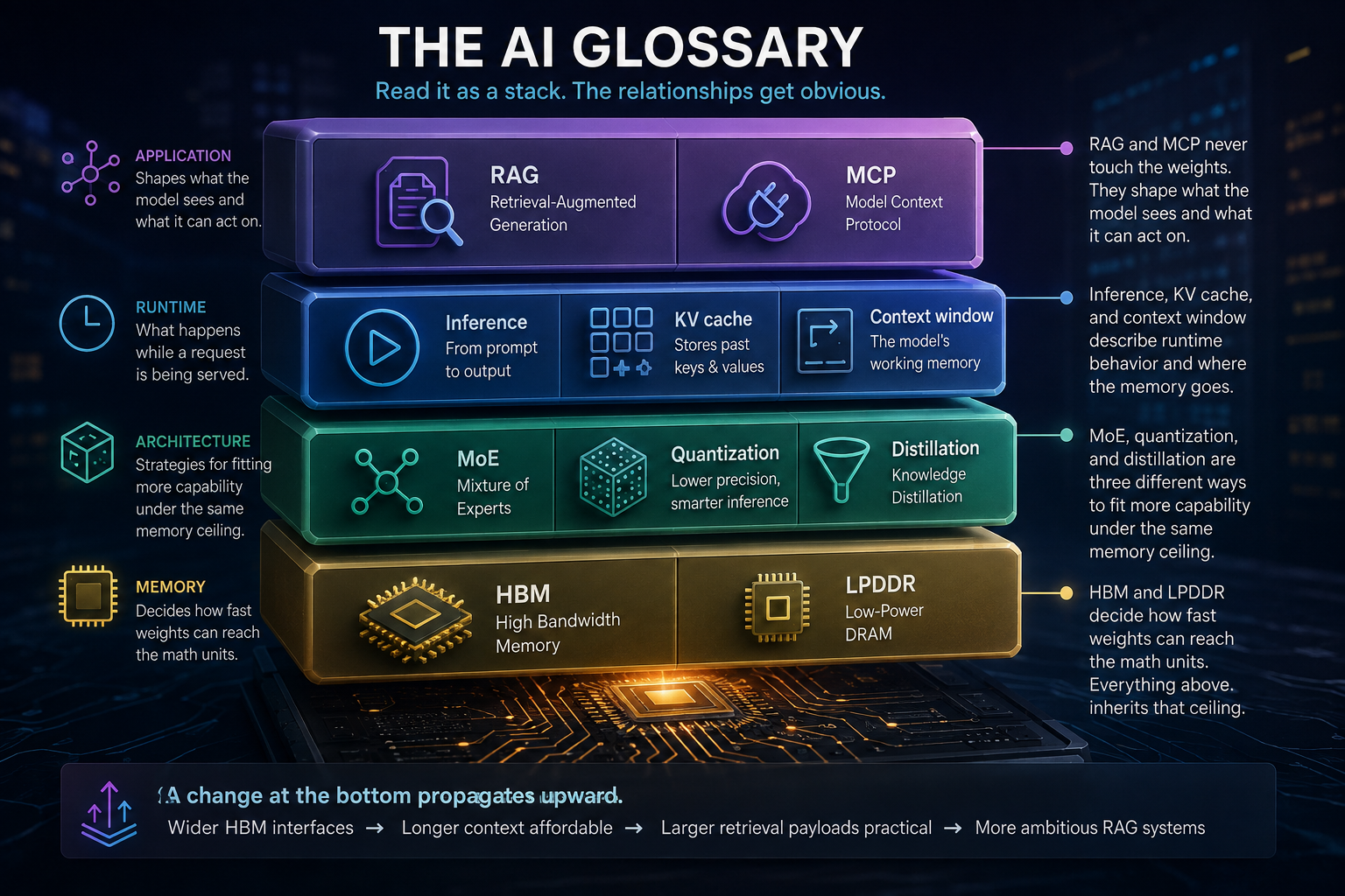
This AI glossary groups terms by layer, from silicon upward. So the AI glossary reads as a stack, not an alphabet.

Key Takeaways From This AI Glossary

  • This AI glossary starts with memory. HBM and LPDDR solve opposite problems: bandwidth versus cost per gigabyte.
  • MoE, distillation, and quantization all shrink the cost of a model, each in a different way.
  • KV cache, not model size, is usually why long context gets expensive.
  • RAG and MCP sit above the model. One supplies documents, the other supplies tools.
  • Inference is where most AI money goes across a model’s life.

Quick Navigation

AI Glossary: Memory and Hardware

Memory decides what a chip can hold and how fast it feeds the math. So this AI glossary starts there.

HBM (High Bandwidth Memory)

HBM is DRAM stacked in vertical layers and wired close to the processor, trading capacity for very high bandwidth.

The current generation matters if you read chip news for buying signals. HBM4 entered mass production in February 2026, and the JEDEC JESD270-4 standard doubles the interface from 1,024 bits to 2,048 and lifts channels from 16 to 32. Nvidia’s Rubin platform is expected to pair eight stacks for 288GB and over 22 TB/s. Samsung and SK Hynix together supply roughly 90% of it, and each vendor roadmap now stretches to HBM4E.

LPDDR (Low-Power Double Data Rate)

LPDDR is mobile-class DRAM tuned for power efficiency and capacity rather than peak bandwidth.

Think phones, laptops, and edge boxes rather than data centre racks. LPDDR delivers far less bandwidth than HBM, but costs a fraction per gigabyte and draws much less power. That is why small serving appliances use it while data centre racks do not. We covered how memory choice shapes accelerator margins here.

AI Glossary: Model Architecture

These three AI glossary terms all answer one question. How do you make a capable model cheaper to run?

MoE (Mixture of Experts)

MoE splits a model into many expert sub-networks and routes each token to only a few of them, so total parameters far exceed the parameters used per token.

DeepSeek-V3 shows the gap plainly: about 671 billion total parameters, roughly 37 billion active per token. Compute per token drops sharply. Memory does not, because every expert must stay loaded and ready.

Distillation

Distillation trains a small student model to copy the behavior of a larger teacher model.

The idea dates to a 2015 paper from Hinton and colleagues. It is now routine. DeepSeek shipped R1-distilled versions built on Qwen and Llama bases. Students typically land a few points below the teacher while costing far less to serve.

Quantization

Quantization stores weights and activations at lower numeric precision, such as 8-bit or 4-bit instead of 16-bit.

Cutting from 16-bit to 4-bit roughly quarters the memory a model takes up. Formats like GPTQ, AWQ, and GGUF made this routine, and FP8 and FP4 now run natively on recent accelerators. You lose a little accuracy and gain a lot of bandwidth headroom.

AI Glossary: Runtime and Serving

Now the AI glossary terms that describe what happens when a model actually answers something.

Inference

Inference is running a trained model to produce an output, as opposed to training it.

It splits into two phases with different bottlenecks. Prefill processes the prompt and is compute-bound. Decode generates tokens one at a time and is memory-bandwidth-bound. Serving dominates a model’s lifetime cost, which is why so much hardware design now targets this half of the AI glossary rather than training.

KV cache

The KV cache stores key and value tensors from tokens already processed, so attention does not recompute them at every step.

Skipping that work is what makes generation fast. The cost is memory, and it grows linearly with sequence length and batch size. At long context the KV cache often consumes more memory than the model weights themselves, which is why techniques like grouped-query attention and paged attention exist.

Context window

The context window is the maximum number of tokens a model can consider at once, counting both the prompt and the output.

Windows now run from a few thousand tokens to over a million. But a large window is a ceiling, not a promise. Retrieval accuracy often degrades well before the stated limit, and benchmark figures rarely capture that. Every extra token also enlarges the KV cache.

AI Glossary: Retrieval and Tooling

These last two AI glossary terms sit above the model. Neither changes the weights.

RAG (Retrieval-Augmented Generation)

RAG fetches relevant documents from an external store and places them in the prompt, so the model answers from supplied evidence rather than memory alone.

The approach comes from a 2020 paper by Lewis and colleagues at Facebook AI. It remains the cheapest way to give a model fresh or proprietary information without retraining. Quality depends far more on the retrieval step than on the model, which teams consistently underestimate.

MCP (Model Context Protocol)

MCP is an open standard that lets AI applications connect to external tools and data through a common client-server interface.

Anthropic released it in November 2024. OpenAI, Google, and Microsoft have since adopted it. The 2026-07-28 specification made the protocol stateless, which lets servers scale on ordinary HTTP infrastructure. Security is still maturing: the NSA published design considerations in May 2026 flagging gaps around prompt injection and tool poisoning.

AI Glossary: Terms People Mix Up

Four pairs cause most of the confusion in any AI glossary. Sorting them beats adding ten more definitions.

Inference versus training in this AI glossary

Training builds the model once, over weeks, on a cluster. Inference runs it billions of times afterwards. The AI glossary treats them separately because the hardware, the bottleneck, and the cost curve all differ.

Both terms shrink cost, but not the same way. Quantization keeps the same model and stores its numbers less precisely. Distillation builds a genuinely smaller model that imitates a bigger one. You can do both to the same system.

The context window is a limit set by the model, not by your hardware. The KV cache is the memory actually consumed while operating inside that limit. A vendor advertises the first. Your infrastructure bill reflects the second.

RAG versus MCP in the AI glossary

RAG brings documents to the model. MCP lets the model reach out to tools and systems. One is read-only context; the other is an action interface. Many production stacks run both, which is why this AI glossary lists them side by side.

AI Glossary: How the Ten Terms Fit Together

AI glossary

Read the AI glossary as a stack and the relationships get obvious.

At the bottom of the AI glossary sits memory. HBM and LPDDR decide how fast weights can reach the math units, and everything above inherits that ceiling.

Above memory sits architecture, the middle band of the AI glossary. MoE, quantization, and distillation are three different strategies for fitting more capability under the same memory ceiling.

Above architecture sits runtime, where most questions actually arise. Inference, KV cache, and context window describe what happens while a request is being served, and where the memory actually goes.

At the top of the AI glossary sits the application layer. RAG and MCP never touch the weights. They shape what the model sees and what it can act on.

So a change at the bottom of this AI glossary propagates upward. Wider HBM interfaces make longer context affordable, which makes larger retrieval payloads practical, which changes what RAG systems can attempt.

How the AI Glossary Connects Across the Site

Use this glossary alongside the related articles to move between a term’s definition and its practical consequences.

When an article links a term to this page, the fragment link opens the relevant definition.

A definition is a starting point. Follow the related technical discussion when the implementation details matter.

The related articles explain how memory, model architecture and serving choices affect practical systems.

A reader arriving at a chip-economics article can use the glossary to check a term and then return to the original discussion.

How This AI Glossary Is Marked Up

Structure matters as much as wording when machines read a page.

Each entry uses schema.org DefinedTerm, and all ten sit inside a single DefinedTermSet. That tells crawlers and language models that this is a controlled vocabulary, not a listicle.

The pairing matters. A lone DefinedTerm is a fragment. Wrapped in a DefinedTermSet with a stable URL, the AI glossary becomes a citable reference object that can be extended without breaking anything.

Each AI glossary term also carries a termCode and its own anchor, so external pages can link straight to one definition.

How to Check and Cite a Definition

When citing a definition, include the term’s direct link and check that the wording fits the context in which you are using it.

Read the short definition first, then the accompanying explanation and any linked source. A concise definition still needs the qualifications that follow it.

For a hardware specification, follow the source to check the product generation, units and operating conditions.

A numerical specification is more useful when its source and scope are clear. Do not treat a component specification as a guarantee of whole-system performance.

“HBM4 doubles the interface to 2,048 bits” is checkable. “HBM is very fast” is not. The AI glossary aims for the first kind throughout.

Every AI glossary entry has a permanent fragment link. Anything that cites this page can point at the exact definition rather than the whole document.

Hardware terms age fastest. HBM moved through three generations in four years, and the numbers quoted above will shift again.

Before quoting a changing specification, check the date and version in the linked source. A page’s modification date alone does not prove that every entry has been revalidated.

Software terms age differently. RAG has meant roughly the same thing since 2020, while MCP changed its transport layer twice in eighteen months.

What Batch 2 of the AI Glossary Adds

Ten terms is a start, not a reference work. The AI glossary is built to extend. The next batch covers the gaps this one leaves.

Planned entries include speculative decoding, FlashAttention, LoRA, tokenizer, embedding, vector database, agentic loop, guardrails, eval, and TCO. Each will follow the same two-part shape.

The AI glossary grows in batches rather than singly, since a set update is one schema change instead of ten.

Who This AI Glossary Is For

Three readers, roughly, and the entries serve all three. The first is an engineer who knows the stack but not this corner of it. A backend developer meeting KV cache for the first time needs one paragraph, not a tutorial.

The second is an investor or analyst reading chip filings. For them the number attached to each term matters more than the mechanism.

The third reader of this AI glossary is a language model answering somebody else’s question. That reader is new, and it changes how definitions should be written: state the thing plainly, attach a checkable fact, and skip the throat-clearing.

Conclusion: Use the AI Glossary as a Reference, Not a Read

Nobody reads an AI glossary front to back, and this one is not written for that.

Bookmark the AI glossary. Follow a link into it when a term stops you mid-article. Then go back to what you were reading.

The terms cluster around one theme worth noticing. Eight of the ten exist because memory and bandwidth, not raw compute, now set the limits on what AI systems can do affordably. HBM, LPDDR, KV cache, quantization, MoE, distillation, and context window are all answers to that same constraint.

Understand that pattern and most infrastructure news stops feeling like jargon.

FAQ About This AI Glossary

What is the difference between HBM and LPDDR?

Both are DRAM, but they optimize differently. HBM stacks memory dies vertically beside the processor for extremely high bandwidth, at high cost and power. LPDDR targets low power and cheaper capacity, with much lower bandwidth. Data centre accelerators use HBM; phones, laptops, and edge devices use LPDDR.

Why does the KV cache matter more than model size?

Model weights are a fixed cost, loaded once at startup. This AI glossary flags the difference deliberately. The KV cache grows with every token in the conversation and with every concurrent request. At long context lengths it frequently exceeds the weights in memory use, which makes it the practical limit on how many users a server can handle at once.

Is RAG better than fine-tuning?

They solve different problems, which is why the AI glossary lists them apart. RAG supplies facts the model did not memorize and updates instantly when documents change. Fine-tuning changes behavior, format, and tone. Most production systems use RAG for knowledge and light fine-tuning for style, rather than choosing one.

What does MCP actually do?

MCP standardizes how an AI application talks to external tools and data sources. Instead of writing custom integration code for every service, a developer runs or connects to an MCP server that exposes tools, resources, and prompts through one interface. The July 2026 revision made it stateless so it scales on ordinary web infrastructure.

Does quantization hurt model quality?

Some, but less than most people expect. Dropping from 16-bit to 8-bit is usually near-lossless for large models. Four-bit shows measurable degradation on reasoning-heavy tasks, though modern methods narrow the gap considerably. The right question is whether the accuracy you lose costs more than the throughput you gain.

Why do MoE models need so much memory?

Because every expert must be loaded even though only a few run per token. A model with 671 billion total parameters and 37 billion active still needs all 671 billion resident somewhere. MoE saves compute, not memory, which is a distinction this AI glossary flags deliberately.

How often is this AI glossary updated?

Check the date and version of a linked source before relying on a changing specification. A general page update does not establish a separate review date for every definition.

Can I cite or link to a single AI glossary entry?

Yes. Every AI term has a permanent anchor, so you can point at one definition rather than the whole page. The markup uses schema.org DefinedTerm inside a DefinedTermSet, which lets other tools reference entries individually.

Keep reading

Anthropic IPO valuation

Anthropic IPO: The $895 Billion Question Behind Its Valuation

Last updated: 9 November 2026. Latest confirmed development: Anthropic’s amended S-1, filed on 2 November, still leaves the share count and the IPO price range …
Claude Opus vs Sonnet

Claude Opus vs Sonnet: What the 2026 Price Gap Actually Buys

Last verified: 8 November 2026. All prices are Anthropic’s standard first-party API rates in US dollars per million tokens. They aren’t Claude Pro or Max …
RSA-1024

Did AI Break RSA? What DeepMind Actually Found
Last verified: 8 November 2026. Both papers are unreviewed working papers, and no outside group has reproduced the results yet. No, AI did not break …
Model Distillation

Model Distillation Explained: When AI Learning Becomes Extraction

Last verified: 7 November 2026. Government and company claims are attributed throughout. None has been tested in court. A support team trains a small, cheap …