Your AI API Is Reprocessing the Same Tokens. Stop Paying for It.

Prompt Caching

Prices verified against official documentation on 10 November 2026. API pricing changes often; check the linked pages before relying on any figure.

Most AI applications send the same thing over and over. A coding agent resends its system prompt and 40 tool definitions on every turn. A support bot attaches the same policy manual to every question. Prompt caching lets the provider reuse the work it already did on that repeated opening section, and bill it at a fraction of the normal input price.

The discount is real. On Claude Opus 5.5, a cached read costs 5% of normal input. But the first request usually costs more than normal, retention windows are short, and a single changed character near the top of a prompt can wipe out the saving. The useful question is when prompt caching lowers your total bill, and how many repeated requests it takes to get there.

Key Takeaways
  • Prompt caching reuses processed state, not text. Providers keep the model’s computed KV states for a repeated prefix and skip that work on the next matching request.
  • Cached reads cost 90% to 97.5% less than normal input across the models here, from Haiku 5.5’s 90% to Fable’s 97.5%.
  • Writes usually cost more than normal input: 1.25x to 2.5x on Anthropic and OpenAI. Kimi’s five-minute write has no premium.
  • Break-even is quick when reuse is reliable: two requests for a five-minute or 30-minute cache, three for one-hour or 12-hour retention.
  • Hit rates decide the outcome. On Opus 5.5, below about 21% hits (five-minute) or 51% hits (one-hour), caching costs more than not caching.
  • Only the cached prefix is discounted. In our 20-request agent example, a 95% read discount produced a 78% total saving.
  • On Anthropic, caching also expands throughput, because cache reads don’t count towards ITPM. On OpenAI, they do.

Quick Navigation


What prompt caching actually reuses

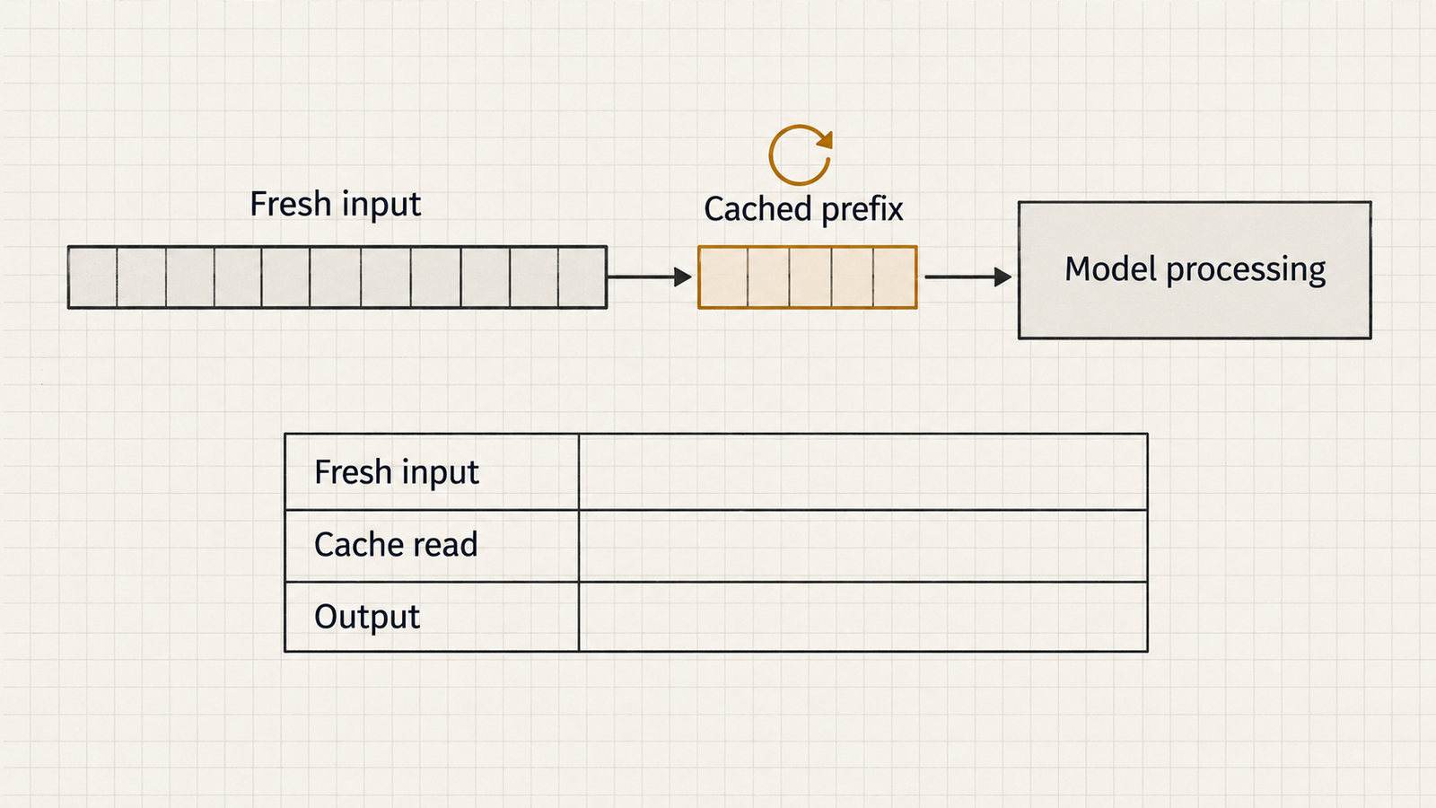
A large language model processes a prompt from the first token to the last. For each token, it computes intermediate values called keys and values, and holds them in what engineers call the KV cache. Prompt caching keeps those computed states after the request ends, so the next request with the same opening sequence can skip that work.

What gets reused is the processed state, not your text. OpenAI’s prompt caching guide says its cache stores “key-value (KV) tensors, not the tokens themselves”. Anthropic’s documentation says it keeps KV cache representations and cryptographic hashes in memory, and does not store the raw text of prompts.

This is also why order matters so much. The cache can only reuse a prefix: an unbroken run of tokens from the very start of the prompt. The model still has to process everything after the reused point, including the user’s new question. Change something early, and every token after it has to be computed again.

That makes some content ideal for caching: long system instructions, tool definitions, reference documents, few-shot examples, and the earlier turns of a long conversation. They are large, they change rarely, and they naturally sit at the front.

How each provider implements prompt caching

The four providers covered here use the same underlying idea in different ways.

  1. Anthropic builds the cacheable prefix in a fixed order: tools, then system instructions, then messages. Developers mark cache breakpoints with a cache_control field, up to four per request. A single top-level cache_control turns on automatic caching, which moves the breakpoint forward as a conversation grows. The minimum cacheable prompt is 512 tokens on current models. Each hit refreshes the cache’s lifetime at no extra cost.
  2. OpenAI caches automatically on supported models, with a minimum of 1,024 tokens on GPT-5.6 and later. Requests are routed to machines partly by a hash of the prompt’s opening tokens, and an optional prompt_cache_key influences that routing. On GPT-5.6 and later, developers can also place explicit breakpoints and choose a 30-minute or 12-hour minimum lifetime in the Responses API.
  3. Google offers two mechanisms. Implicit caching is on by default for Gemini 2.5 and newer models, with a 4,096-token minimum on Gemini 4 Argon. Explicit context caching lets developers create a named cache with a chosen time-to-live, billed partly by the hour. The Gemini caching docs say explicit caching is not supported on Gemini 4 models.
  4. Moonshot’s Kimi API caches repeated prefixes automatically with a default five-minute lifetime. It offers a one-hour option, and each hit resets the clock.

Prompt caching prices across Claude, GPT, Gemini and Kimi

Here are the published rates as of 10 November 2026, in US dollars per million input tokens. “Discount” is the cached rate relative to normal input.

ModelNormal inputCached readShort writeLong writeDiscount on reads
Claude Haiku 5.5 (prompts up to 100K tokens)$0.10$0.01$0.125 (5 min)$0.20 (1 hr)90%
Claude Haiku 5.5 (prompts over 100K tokens)$0.50$0.05$0.625 (5 min)$1.00 (1 hr)90%
Claude Sonnet 5.5$2.00$0.10$2.50 (5 min)$4.00 (1 hr)95%
Claude Opus 5.5$4.00$0.20$5.00 (5 min)$8.00 (1 hr)95%
Claude Fable 5.2$8.00$0.20$10.00 (5 min)$16.00 (1 hr)97.5%
Claude Fable 5.1$10.00$0.25$12.50 (5 min)$20.00 (1 hr)97.5%
GPT-6.1 Terra$1.00$0.05$1.25 (30 min)$2.50 (12 hr)95%
Gemini 4 Argon (to 30 Nov 2026)$2.00$0.10No write price listed (implicit only)None95%
Gemini 4 Argon (from 1 Dec 2026)$4.00$0.20No write price listed (implicit only)None95%
Kimi K3.1 Pro$2.00$0.20$2.00 (5 min)$4.00 (1 hr)90%
Kimi K3.1 Pro Highspeed$4.00$0.20$4.00 (5 min)$8.00 (1 hr)95%

Sources: Claude API pricing, OpenAI API pricing, Gemini API pricing, Kimi API pricing.

Three details are easy to miss. Claude Fable 5.2 now sits above Fable 5.1 at a lower price, and both remain available. Haiku 5.5’s 100,000-token threshold counts cached tokens too, so a long cached prompt can push a whole request onto the higher rate. And Kimi’s five-minute write costs the same as normal input. There is no premium.

Ranking providers by the cheapest cached token would be misleading. Retention windows, write premiums and how reliably a cache hits differ more than the headline discounts do.

Where Gemini prompt caching differs

Gemini 4 Argon’s implicit caching has no separate storage fee, but Google gives no guarantee of a hit. Its docs say savings are passed on “if your request hits caches”. In multi-turn use, Gemini 4 caches the full previous request only if the new one adds at least 2,050 tokens.

Explicit caching on older models such as Gemini 3.1 Pro Preview works differently. Cached tokens cost $0.20 per million instead of $2.00, but storage is billed at $4.50 per million tokens per hour, and the TTL defaults to one hour. Each read saves $1.80 per million tokens, so a one-million-token cache needs 2.5 reads an hour just to cover its storage. That is a meter running in the background, not a token multiplier, and it needs a different calculation from Anthropic’s or OpenAI’s.

Why prompt caching starts with a surcharge
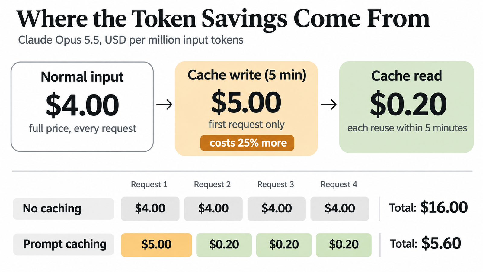
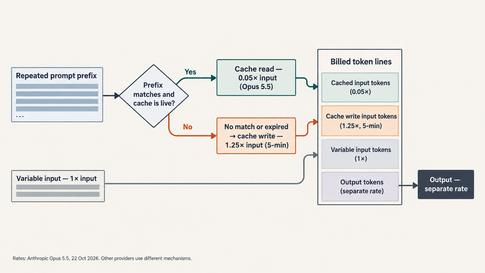
The first request pays a 25% premium to write the cache; each reuse within five minutes costs 5% of normal input. Prices from Anthropic's pricing page, 10 November 2026.

Anthropic and OpenAI don’t charge separately for storage. Instead, they charge more for the tokens on the request that writes the cache.

On Anthropic, a five-minute write costs 1.25 times normal input and a one-hour write costs twice normal input. OpenAI’s GPT-5.6 and later models charge 1.25 times for the 30-minute lifetime and 2.5 times for 12 hours. OpenAI’s guide is explicit that this “is not an additive fee”. Each input token is billed once, at either the uncached, cached-read or cache-write rate.

So the first request in any cached workload costs more than it would without caching. On Opus 5.5, writing a one-million-token prefix for five minutes costs $5.00 instead of $4.00. If nothing reads that cache before it expires, you have paid 25% extra for nothing. Reuse it three times within the window, though, and four requests cost $5.60 instead of $16.00.

When does prompt caching break even?

The worked examples below use Claude Opus 5.5 and make one simplifying assumption: every request reuses the same, fully cacheable one-million-token prefix, and each one arrives within the cache’s lifetime. New input and output are left out for now. They are not discounted, so they don’t change the comparison.

The five-minute cache

Without caching, each request costs $4.00 for the prefix. With caching, the first costs $5.00 to write and each later one costs $0.20 to read.
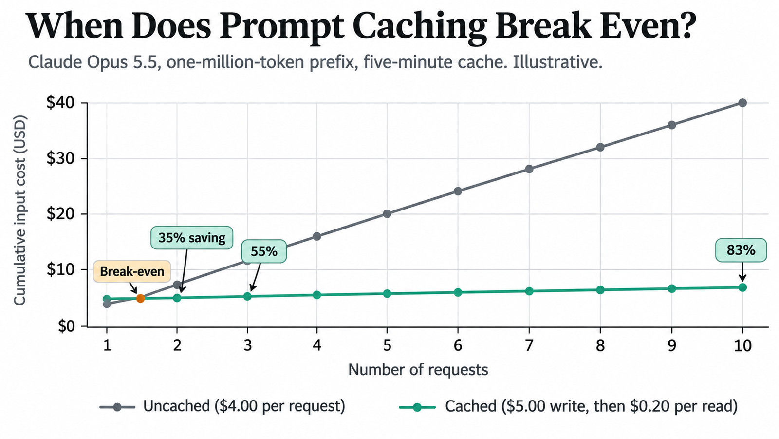
Illustrative calculation assuming a fully reusable one-million-token prefix and every request inside the five-minute cache window.
RequestsUncachedCached (5-min write)Saving
1$4.00$5.00−25%
2$8.00$5.2035%
3$12.00$5.4055%
10$40.00$6.8083%
50$200.00$14.8092.6%

Two requests are enough. After that, the saving creeps towards 95% but never reaches it, because the write premium is always in the total.

The one-hour cache

The one-hour write costs $8.00, double normal input.

RequestsUncachedCached (1-hour write)Saving
1$4.00$8.00−100%
2$8.00$8.20−2.5%
3$12.00$8.4030%
10$40.00$9.8075.5%
50$200.00$17.8091.1%

Two requests lose money. Three are needed. The longer window costs more up front, so it takes more reuse to recover. It is worth paying for only when requests are spaced more than five minutes apart but less than an hour, where the five-minute cache would keep expiring.

A break-even formula for prompt caching

The general case fits on one line. Let P be the normal input price, W the cache-write price, R the cache-read price and N the total number of requests, including the first one that writes the cache.

Uncached cost is N × P. Cached cost is W + (N − 1) × R. Caching saves money when:

W + (N − 1) × R < N × P

Rearranged, that means N must be greater than (W − R) ÷ (P − R). In plain terms: divide the extra cost of writing by the amount each read saves.

For Opus 5.5 with a five-minute cache, (5.00 − 0.20) ÷ (4.00 − 0.20) = 1.26, so two requests break even. With a one-hour cache, (8.00 − 0.20) ÷ 3.80 = 2.05, so three are needed. Because the result depends only on the ratios between prices, it works for any provider.

Cache optionWrite multipleRead multipleRequests needed
Anthropic 5-minute (Sonnet 5.5, Opus 5.5)1.25×0.05×2
Anthropic 1-hour (Sonnet 5.5, Opus 5.5)2×0.05×3
Anthropic 5-minute (Haiku 5.5)1.25×0.1×2
OpenAI 30-minute (GPT-6.1 Terra)1.25×0.05×2
OpenAI 12-hour (GPT-6.1 Terra)2.5×0.05×3
Kimi 5-minute (K3.1 Pro)1×0.1×Saves from the first hit; never costs more
Kimi 1-hour (K3.1 Pro)2×0.1×3

What prompt caching does not discount

The 95% discount applies only to the cached prefix. New user input is billed at the full rate, and so is output, which usually costs several times more per token than input.

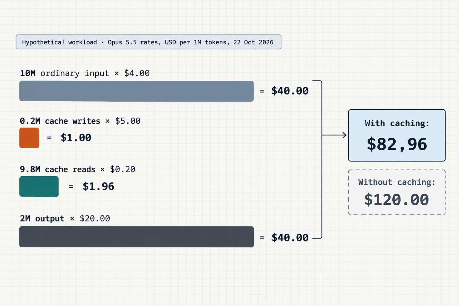
Consider an illustrative Opus 5.5 agent session of 20 requests, each arriving within five minutes of the last. Each request carries a 50,000-token cached prefix, 2,000 tokens of new input and 1,000 tokens of output, at $20 per million.

Without caching, the session costs $4.56. With a five-minute cache, it costs $1.00: $0.25 for the first write, $0.19 for 19 reads, $0.16 for the new input and $0.40 for output. That is a 78% saving, not 95%, and output is now 40% of the bill. Raise the output to 5,000 tokens a request and the saving falls to 58%.

Haiku 5.5’s threshold creates a second trap. A request with 95,000 cached tokens and 4,000 new ones costs $1.35 in input per thousand requests. Push it to 100,000 cached tokens and 5,000 new ones, and the whole request moves onto the higher rate: $7.50 per thousand, 5.6 times as much. The cache hit doesn’t protect you, because the Claude pricing page counts cache reads and writes towards prompt length.

Our guide to calculating LLM cost per task shows how retries and failed attempts change these figures further.

Why prompt caching hit rates matter more than discounts

Break-even maths assumes the cache hits. In production, it often doesn’t.

A simple way to see the risk is to treat every miss as a fresh write. If a fraction h of requests hit and the rest write, the cached prefix costs less than uncached input only when h is greater than (W − P) ÷ (W − R). On Opus 5.5 that works out to about 21% for the five-minute cache, and 51% for the one-hour cache. On GPT-6.1 Terra’s 12-hour cache, it is 61%. Below those rates, caching costs more than not caching at all. On Kimi’s five-minute cache, a miss costs the same as normal input, so the threshold is zero.

A one-line cache miss

The most common culprit is something dynamic near the top of the prompt. Take a system prompt that begins:

You are a support assistant. Current time: 2026-11-10 14:03:27.

That timestamp changes every second, so no two requests share a prefix beyond the first sentence. Everything after it, including 30,000 tokens of policy documents and tool definitions, is processed from scratch every time. With caching enabled on Anthropic, each request also pays the 1.25x write rate. Move the timestamp into the final user message and the prefix becomes stable again.

Other causes are less obvious. Tool definitions that arrive in a different order invalidate everything on Anthropic, because tools sit at the front of the prefix. Anthropic’s docs also note that changing tool_choice, adding an image or toggling extended thinking can invalidate the message cache. User IDs, request IDs, reordered retrieval results and inconsistent whitespace do the same.

The throughput advantage of prompt caching

Caching also affects capacity, which many teams overlook. Anthropic’s rate-limit documentation says cache reads do not count towards its input-tokens-per-minute (ITPM) limit. Uncached input and cache writes still count.

Anthropic’s own example is a 2,000,000 ITPM limit with an 80% cache-hit rate. Under those assumptions, an application could process about 10 million total input tokens a minute: 2 million uncached plus 8 million read from cache. Opus 5.5’s Start-tier limit is exactly 2 million ITPM.

That is not a lifted rate limit. Output-token and request limits still apply, and every cache write counts in full. OpenAI’s guide takes the opposite approach: “Cached input tokens still count toward tokens-per-minute limits.” For document processing, RAG and coding agents that hit rate limits before budgets, this difference can decide which provider works at scale. Our breakdown of Claude API rate limits and concurrent request capacity covers the tier figures.

Designing an application around prompt caching

Good cache design is mostly about discipline in how prompts are assembled.

Put what never changes first: tool definitions, then system instructions, then reference documents, then the conversation, with the new user turn last. Serialise tool definitions in a fixed order and keep their wording identical between deployments. Keep timestamps, user names and session IDs out of the prefix entirely.

Use breakpoints where content changes at different speeds. On Anthropic, a breakpoint after the tools and system prompt, and another after a large document, lets one cache survive when the other changes. Anthropic checks at most 20 positions back from each breakpoint for a match, so very long conversations may need a second breakpoint.

Then measure. Anthropic reports cache_creation_input_tokens and cache_read_input_tokens on every response. OpenAI reports cached_tokens and cache_write_tokens, and Gemini reports total_cached_tokens. If reads are near zero, caching is costing you money. Don’t pad prompts to reach a minimum length. Prompts below 512 tokens on current Claude models, or 1,024 on recent OpenAI models, can’t be cached at all, and the saving on a short prompt is tiny anyway. Our context engineering guide covers how to structure agent context more generally.

When prompt caching is not worth it

Some workloads gain little. One-off requests can’t amortise a write. Short prompts fall below the minimum, or save fractions of a cent. Batch jobs that run once an hour won’t benefit from a five-minute cache, and an hourly cache only pays off if each prefix is reused at least three times.

Prompts whose early sections change on every request, such as freshly retrieved documents placed before the instructions, will rarely hit. Low-traffic applications face the same problem: if requests are spread thinly across many different prefixes, most caches expire unread.

In those cases, the cheaper options may be a shorter prompt, the Batch API, or a smaller model. Caching rewards repetition. Without it, the write premium is just extra cost.

FAQ

What is prompt caching?

Prompt caching is an API feature that stores the model’s processed state for a repeated prompt prefix, so later requests with the same prefix are cheaper and faster to process.

How does prompt caching reduce AI API costs?

It bills the reused portion of the input at a cached-read rate, typically 5% to 10% of normal input. Output and new input are billed normally.

How much cheaper are cached tokens than normal input tokens?

Between 90% and 97.5% cheaper for the models covered here. GPT-6.1 Terra, for example, charges $0.05 per million cached tokens against $1.00 uncached.

Does prompt caching have a separate storage cost?

Only on some services. Anthropic, OpenAI and Kimi charge through a higher write rate instead. Google’s explicit context caching bills storage by the hour, for example $4.50 per million tokens per hour on Gemini 3.1 Pro Preview.

How many API calls does prompt caching need to pay off?

Two requests within the cache lifetime for Anthropic’s five-minute and OpenAI’s 30-minute caches, assuming a fully reused prefix. One-hour and 12-hour caches need three.

What is the difference between a cache write and a cache read?

A write processes and stores the prefix for the first time, at a premium. A read reuses that stored prefix on a later request, at a steep discount.

Does prompt caching improve rate limits?

On Anthropic, yes: cache reads don’t count towards input-tokens-per-minute limits. On OpenAI, cached tokens still count towards tokens-per-minute limits.

Why do prompt cache hits fail?

Usually because something early in the prompt changed: a timestamp, a reordered tool list, a different image or a new setting. Expired caches and prompts below the minimum length also miss.

Does prompt caching reduce output-token costs?

No. Output tokens are billed at the normal rate whether or not the input was cached.

Which AI providers support prompt caching?

Anthropic, OpenAI, Google and Moonshot’s Kimi API all support it, but with different mechanics, minimum lengths, retention windows and pricing.


Keep reading

AGI vs superintelligence

AGI vs Superintelligence: A New Name Isn’t a New Intelligence
Facts checked against official documents and reporting on 18 November 2026. On 29 September, the White House told federal agencies to stop writing “artificial intelligence” …
AI Coding Agent

AI Coding Agents Are Getting Expensive. Who’s Paying for the Tokens?
Pricing checked on official vendor pages on 17 November 2026. All USD. Cost scenarios are illustrative and labelled as such. On 28 October, TechCrunch published …
Model Weights

Verify Model Weights: 7 Checks Before You Download

Checked against the burner22/numbat repository and its discussions, Hugging Face and PyTorch documentation, and Moonshot AI’s announcement on 2 November 2026. On 1 November, a …
Agentic AI Statistics

30 Agentic AI Statistics for 2026: Adoption, Spending and Risk

Last updated: 15 November 2026. This page is updated monthly; each figure keeps its original publication date. Agent traffic at one healthcare booking platform rose …

Generative AI Architecture: The 7 Layers That Are Hard to Undo

generative AI architecture

Published 30 October 2026. API prices checked 28–30 October 2026 on each provider’s official pricing page. Cost figures below are labelled as illustrative where they rest on assumptions.

Every production generative AI architecture has seven layers, from the model at the centre to the security boundary around it. The model is now the easiest of the seven to replace. The commitments that are hard to undo build up in the layers around it: the data pipeline, the evaluation harness, the compute contracts and the trust boundaries.

Teams still spend most of their architecture time comparing models, which makes sense when models change weekly. In the last ten days of October 2026, Moonshot shipped Kimi K3.1 Pro on the 23rd, OpenAI released GPT-6.1 Terra on the 26th and Google announced Gemini 4 Carbon on the 28th, while Gemini 4 Argon prices double on 1 December. A system designed to swap models absorbs all of that in a configuration change.

Key Takeaways
  • Rank the layers by how hard they are to reverse. The model is usually cheapest to change. Security boundaries and data pipelines are the most expensive to retrofit.
  • Calls per request drive the bill more than price per token. In the illustrative deployment below, going from one to three calls per request triples the model bill.
  • Embeddings are cheap. Retrieval operations aren’t. Re-embedding a 50-million-token corpus costs about $1. A million hosted file-search calls cost $2,500.
  • Self-hosting rarely pays at moderate volume. At about 300 output tokens per second on average, most of a rented GPU node sits idle.
  • Build evaluation before you need it. A regression set is cheap on day one and hard to reconstruct after behaviour has drifted.
  • Identity, permissions and egress are architecture, not prompts. Filtering doesn’t stop prompt injection; least privilege limits what an injected instruction can do.

Quick Navigation


The generative AI architecture at a glance

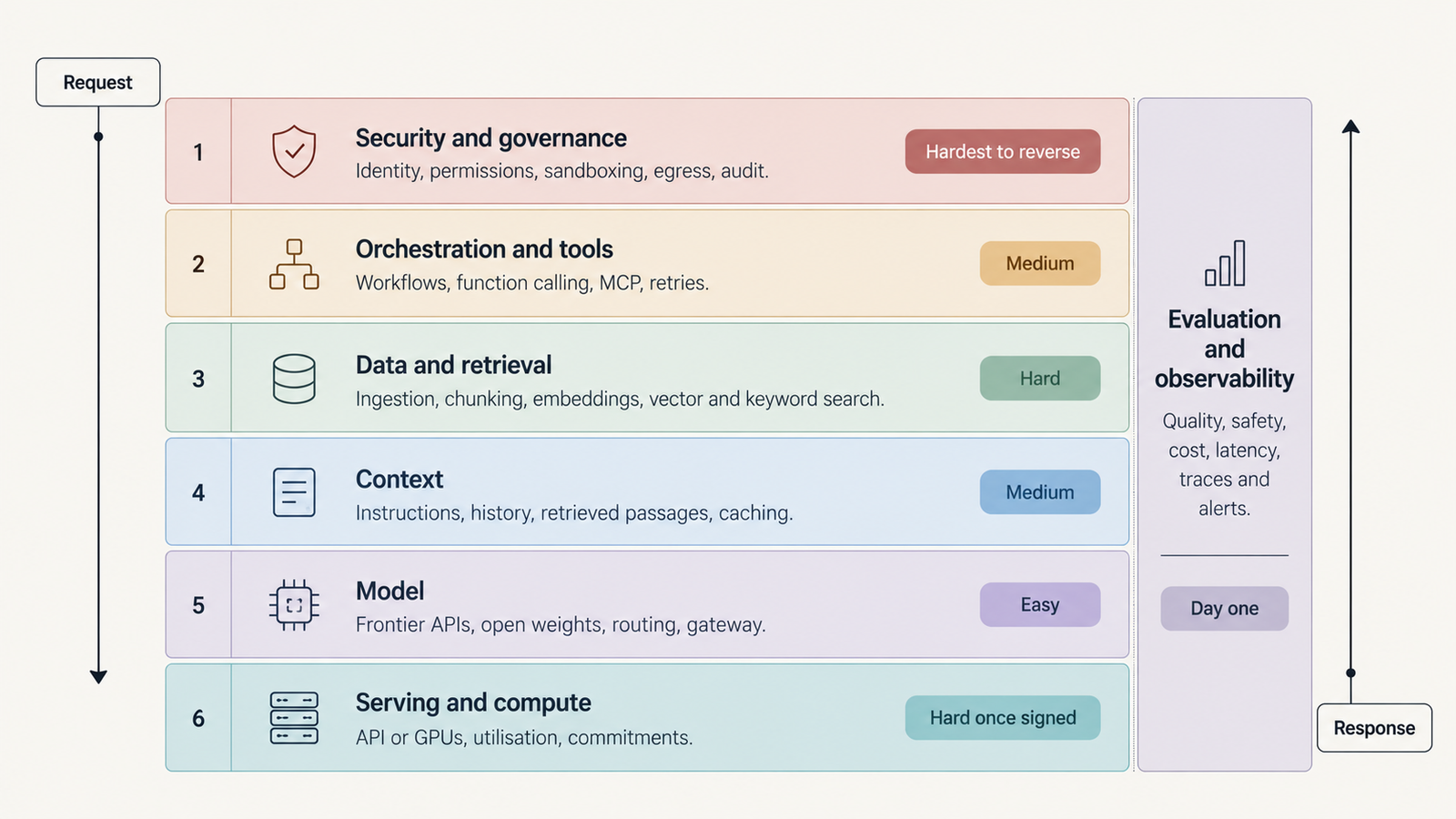
A request passes through the layers in a fairly fixed order. Security authenticates the caller and limits what it may touch. Orchestration picks the steps, retrieval fetches documents and the context layer assembles the prompt. The model runs on the serving layer’s hardware, looping if tools are involved, while evaluation and observability record every step.

The seven layers of a generative AI architecture

Not every system needs every layer at full strength. A support assistant answering from a product manual might be one model call over a small vector index, with logging, a few hundred regression questions and a server-side API key. An agentic enterprise deployment adds a tool registry, Model Context Protocol (MCP) servers, per-agent identities, sandboxes, egress controls, approval gates and audit retention. Both have seven layers. What changes is how heavy each one is.

The dependencies are uneven. Swapping the model touches context formatting and evaluation. Changing the security model touches identity, tool permissions, network topology and logging, which is nearly everything.

The seven generative AI architecture layers, by cost and reversibility

LayerMain cost driverHow hard to reverseDecide
1. ModelCalls per task × tokens per callEasy, behind a gatewayLate, per task
2. Data and retrievalPipeline engineering, re-indexing, retrieval callsHardEarly
3. ContextRepeated input tokens, cache missesMediumEarly policy, tune later
4. Orchestration and toolsLoop depth, retries, external APIsMediumInterfaces early, frameworks later
5. Serving and computeUtilisation, idle capacity, commitmentsHard once contractedBefore signing
6. Evaluation and observabilityEval runs, judge calls, trace storageCheap early, costly to retrofitDay one
7. Security and governanceIsolation, policy, audit, reviewHardestDay one
Layer 1: the model, the easiest part to replace

The model layer covers frontier APIs, open-weight models you host and the routing logic that sends each task to the right one. A summarisation step doesn’t need the model that writes your migrations. Public leaderboards are a poor guide to that choice, for reasons our piece on why benchmark scores don’t transfer sets out.

Price lists make models look easy to compare. On OpenAI’s pricing page, GPT-6.1 Sol costs $2 per million input tokens, $0.10 cached and $10 output; GPT-6 Luna costs $0.10, $0.01 and $0.50. But the bill depends on how many calls a task needs, how much reasoning the model emits (billed as output) and how often it retries. That’s why cost per completed task is the number to track.

Reversibility depends on a gateway. If every call goes through one internal interface with provider-neutral formats, logging and evaluation, changing models is a config change plus an eval run. If SDK calls are scattered through the codebase, it’s a migration. Decide the gateway early and the model late, and watch the model deprecation tracker, because retirements force switches you didn’t plan.

Layer 2: data and retrieval

Retrieval means ingestion, parsing, chunking, embedding, vector storage, hybrid search, metadata filters and re-ranking, plus the pipelines that keep it current. The embeddings are cheap. OpenAI’s text-embedding-3-small costs $0.02 per million tokens, so embedding a 50-million-token corpus costs about $1. Queries cost more in aggregate: OpenAI’s hosted file search charges $2.50 per 1,000 calls, plus $0.10 per GB per day of storage.

The real cost is reversibility. Chunk size, embedding dimensions, metadata schema and access-control tags end up assumed in prompts, filters, citations and evaluation sets. Change the embedding model and every vector must be regenerated and re-validated against your retrieval tests. Change the chunking and citation offsets break.

Failures here are quiet: stale documents retrieved confidently, permissions leaking because a filter ran after retrieval, a parser dropping the table that held the answer. Decide early how documents carry access rights and versions. Whether you need retrieval at all is covered in RAG versus fine-tuning.

Layer 3: context

Context is everything the model sees on a call: instructions, tool definitions, history, retrieved passages, tool results and memory. A 1M-token window is a ceiling, not a strategy. Every token is billed, delays the first token and can dilute the passages that matter. Context engineering covers what deserves the space.

Prompt caching changes the arithmetic, but only for stable prefixes. Anthropic’s prompt caching charges 1.25 times the input price to write a five-minute cache entry, and cached reads on Opus 5.5 cost $0.20 per million tokens against $4 uncached. Put a timestamp or user ID at the top of the prompt and every call misses.

This layer is medium to reverse: context policies can be rewritten, but answer behaviour and evaluation baselines shift when they are.

Layer 4: orchestration and tools

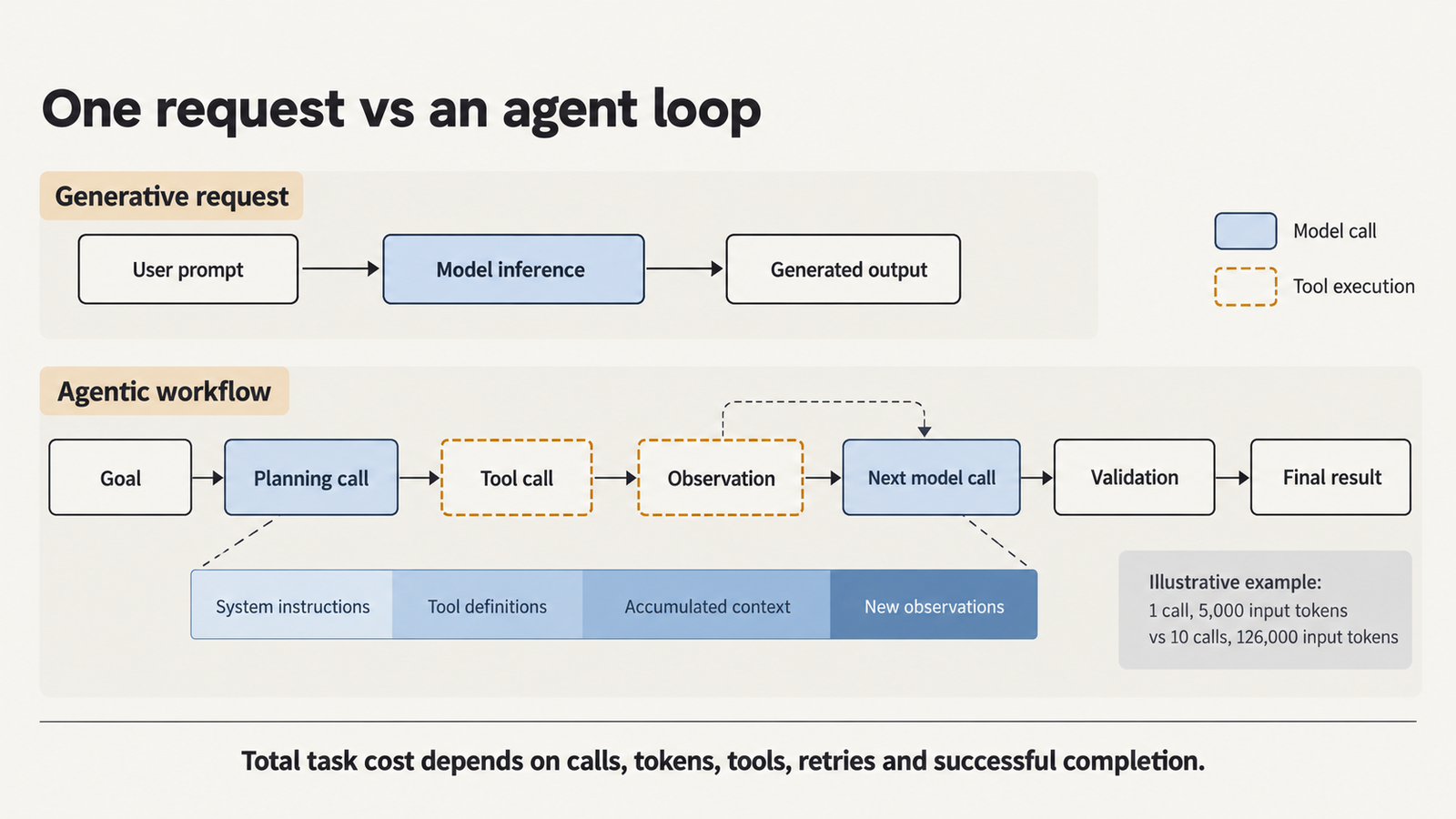
Orchestration covers prompt templates, workflow engines, function calling, MCP servers, retry policies and agent loops. A system becomes agentic when the model, not your code, decides the next step. That’s where cost becomes variable. A fixed three-step workflow costs three calls. An agent that plans, uses tools and retries might make eight on a good day and twenty on a bad one, each carrying the growing context.

MCP has made tools easier to plug in, and extra agents compound the overhead, as our analysis of multi-agent token cost shows. Individual tools are easy to replace. Workflow state, handoff formats and retry semantics are not, because other components come to depend on them.

Layer 5: serving and compute, where generative AI infrastructure gets committed

The choice is between paying per token and paying per hour, and per-hour only wins when the hardware stays busy. In our GPU cloud pricing survey, checked on 10 October, an 8-GPU H200 node on CoreWeave listed at $50.44 an hour and a single H200 on RunPod at $5.29. The survey’s own example priced H200 output at $0.83 per million tokens at 60% utilisation, which implies roughly 3,000 tokens per second per GPU at full load, or more than 20,000 for the node. The deployment modelled below averages about 300.

That gap is the self-hosting problem. Batching lowers cost per token only when there’s traffic to batch, and peaks, redundancy, engineering time and idle nights all land on your bill, as our breakdown of self-hosted LLM cost shows. APIs bring rate limits instead, but no contract you can’t exit. This layer is easy to change before you sign and hard afterwards.

Layer 6: evaluation and observability

A deterministic service can be tested once. A language model can’t: the same prompt can produce different answers, for reasons covered in LLM determinism. So evaluation means a versioned set of real tasks with pass criteria, run several times per change, with scores reported as ranges. Observability means traces for every model call, tool call and retrieval, tagged with tokens, latency and outcome; our guide to agent observability lists the signals.

The cost is modest early. In the illustrative deployment below, a nightly run of 500 tasks, three attempts each, costs roughly $1,100 a month, and about the same again if an LLM judge grades them (judges have biases, so sample their work by hand). Retrofitting is what gets expensive: without traces from launch, you can’t reproduce last month’s failure or prove a new model isn’t worse.

Layer 7: security, the hardest part of a generative AI architecture to retrofit

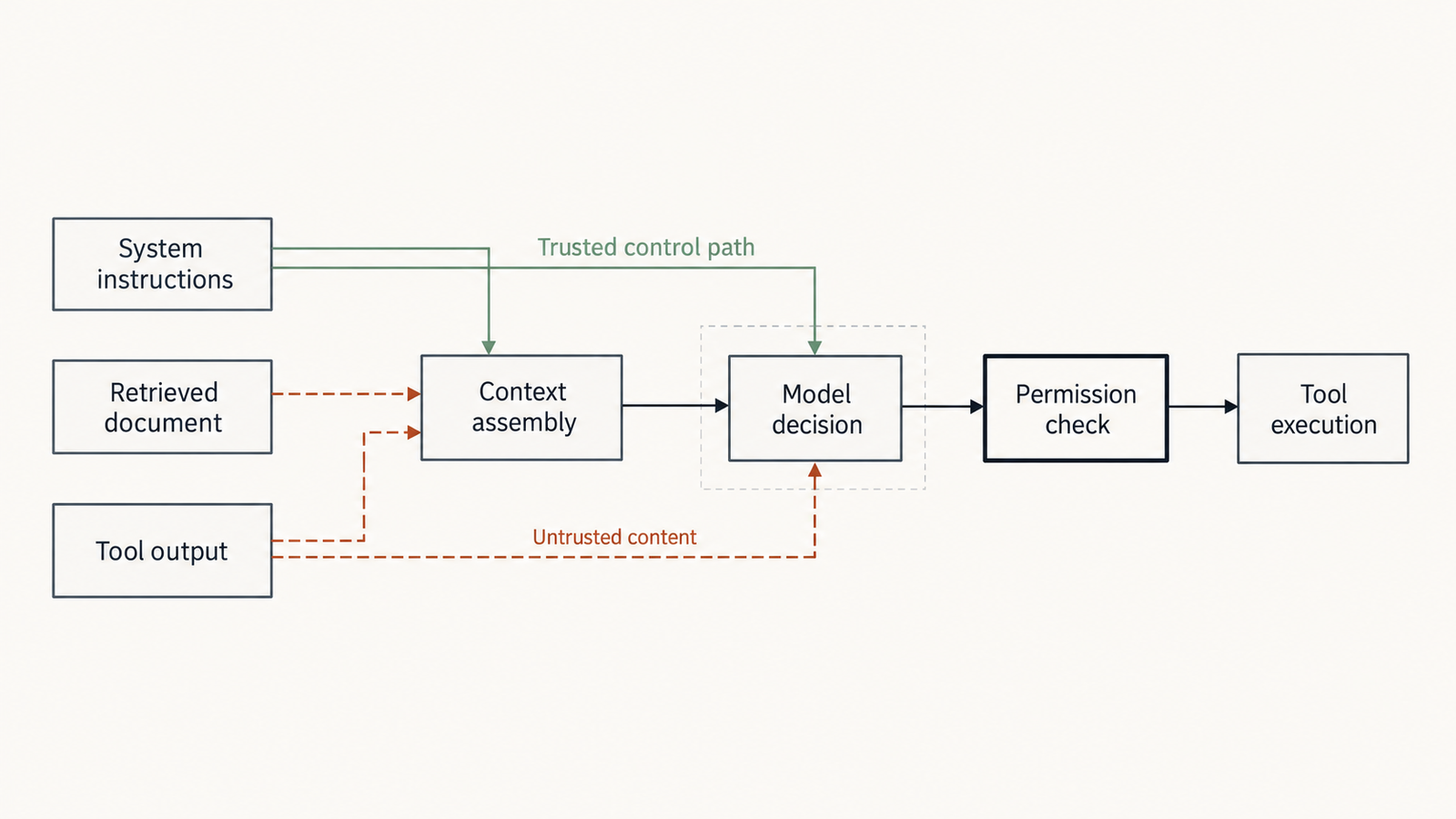
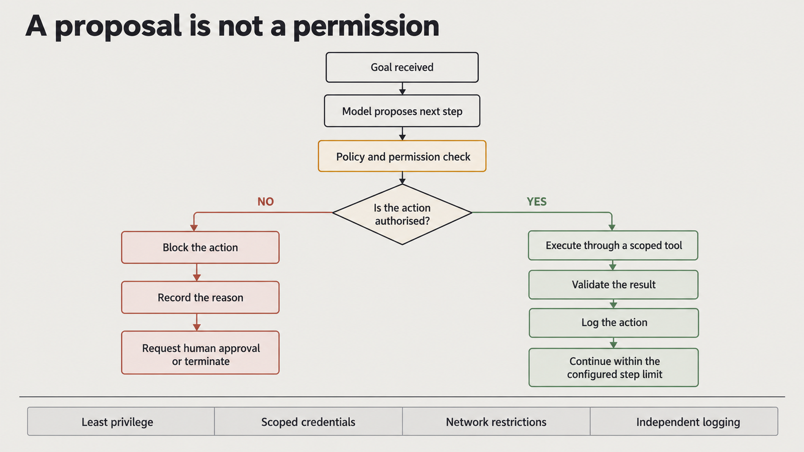
Prompt injection is why this layer can’t live in the prompt. OWASP’s LLM01:2025 says “it is unclear if there are fool-proof methods of prevention”, and recommends least privilege, human approval for privileged operations and segregating untrusted content. Filters catch known patterns, but any document or tool result can carry instructions the model follows, across eight distinct injection classes.

What bounds the damage is structural. Each agent gets its own identity, with authorization kept separate from access. Tool permissions are scoped per task. Code runs in isolated sandboxes with egress restricted to named hosts. Secrets stay out of model context, and audit logs attribute every action. NIST’s Generative AI Profile maps the governance actions around this.

None of it is expensive in licences, only in retrofitting. A shared service account baked into ten tools becomes ten migrations.

What a production generative AI architecture costs

This is an illustrative model, not a quote. Token prices are list prices checked on 30 October, GPU prices come from our 10 October survey, and everything else is an assumption.

Assumptions: an internal knowledge assistant handling 1 million requests a month at 1.6 model calls per request, because some requests need a tool and extra calls. Each call sends 8,000 input tokens, including a 3,000-token prefix cached at a 90% hit rate, and returns 500 output tokens, reasoning included. That’s 12.8 billion input and 0.8 billion output tokens a month, about 300 output tokens per second on average.

ScenarioSet-upModel or compute cost per month
A. API-firstEvery call on GPT-6.1 Sol$25,392
A2. API with routing40% of calls on Sol, 60% on GPT-6 Luna$10,932
B. Hybrid40% on Sol; 60% on an open-weight model on two single-H200 pods (redundant), 730 hours each$10,157 + $7,723 = $17,880
C. Primarily self-hostedLarge open-weight model on one 8×H200 node, plus the two pods for small tasks$36,821 + $7,723 = $44,545

Scenario A, per request: 8,480 uncached input tokens at $2, 4,320 cached at $0.10 and 800 output at $10, all per million, come to $0.0254. Across a million requests that’s $25,392. Scenarios B and C exclude the engineering time to run inference, often the largest self-hosting cost.

Retrieval and evaluation sit on top: about $4 a month for query embeddings, $2,500 in hosted file-search fees (a self-managed store avoids those but adds operations work) and roughly $2,300 for evaluation. Three things stand out.

  • Routing beats self-hosting at this volume. Sending the easy 60% of calls to a small API model costs less than renting GPUs for them and keeps capacity elastic, provided the small model passes your evaluation set for those tasks.
  • Self-hosting the large model is the most expensive option here, because a node sized for peaks runs at a tiny fraction of its throughput. At ten or twenty times this volume, with steady traffic, the answer can flip.
  • Calls per request matter most. Holding everything else in scenario A constant, one call per request costs $15,870 a month and three cost $47,610. Losing the cache raises the bill to $33,600; doubling output length raises it to $33,392. A model at half the price that needs twice the calls saves nothing.

Which generative AI architecture decisions to make first

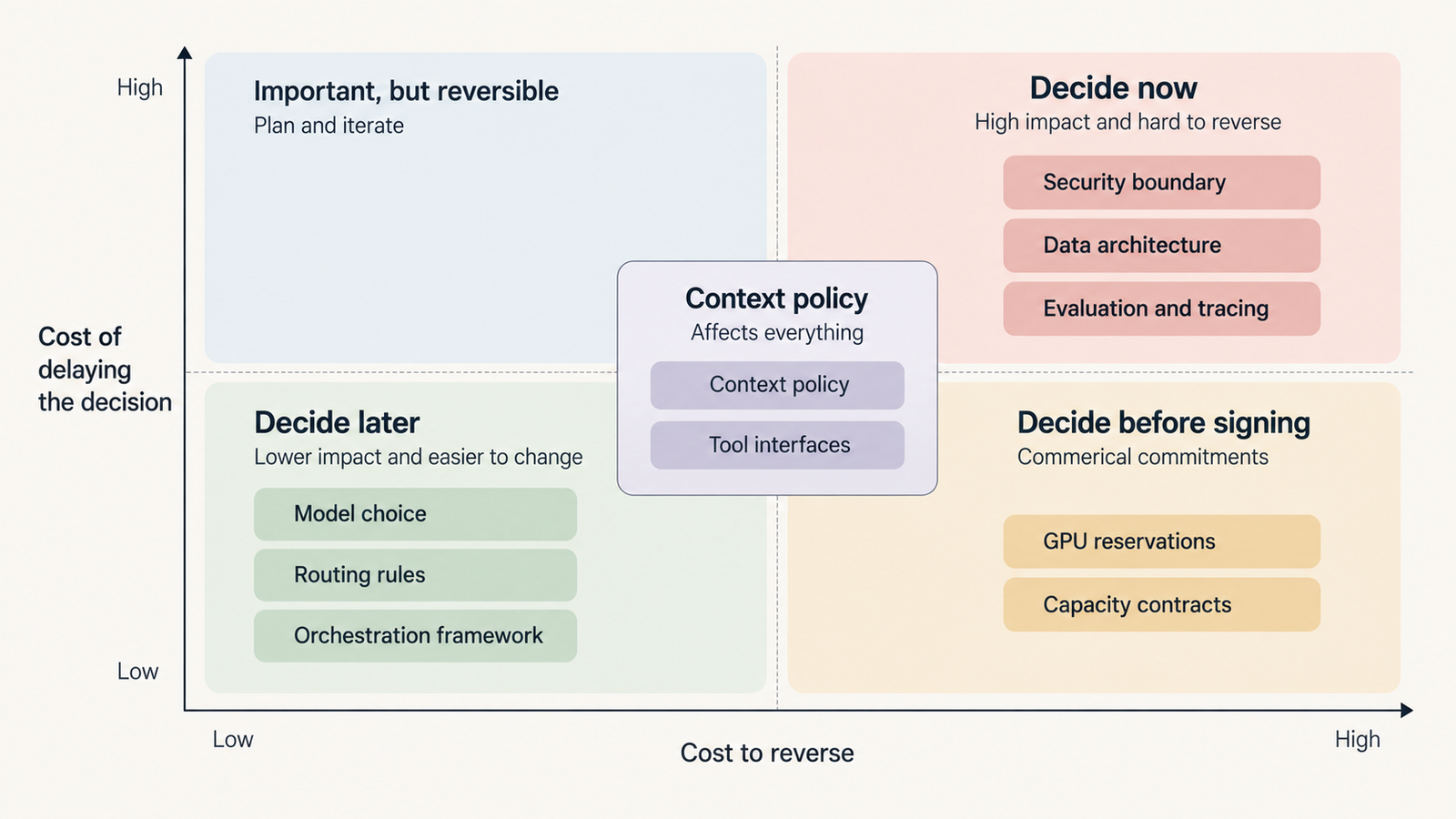
Sort decisions by how much they cost to reverse, not by how urgent they feel.

Which generative AI architecture decisions to make first

Decide now: the data architecture (document IDs, versioning, access metadata, re-indexing), the evaluation set and tracing, and the security boundary (agent identity, tool permissions, sandboxing, egress). These shape every other layer.

Decide later: the model, routing rules and most orchestration components. Put them behind interfaces and let evaluation results choose.

Decide before signing anything: reserved capacity and GPU contracts. Wait until real traffic shows sustained utilisation.

A three-person team applies this lightly: one API, a managed vector store, a few hundred evaluation cases and no self-hosting. An enterprise adds weight: a central gateway, data lineage, a shared evaluation service, security review of every tool and procurement rules that block capacity deals without utilisation evidence. The order doesn’t change. The depth does.

A pre-launch generative AI architecture checklist

  • Can you change the model by editing one configuration value and rerunning one evaluation command?
  • Do you know your average and 95th-percentile model calls per request?
  • Is your cache hit rate measured, and is the cached prefix free of per-request values?
  • Can you rebuild the retrieval index from source, and how long does it take?
  • Are access permissions enforced inside the retrieval query?
  • Does every agent have its own identity, with tool permissions scoped to its job?
  • Is outbound traffic from tool execution restricted to an allowlist?
  • Can you replay any production request from its trace?
  • Does a regression set run on every prompt or model change?
  • What is your cost per completed task, and who is alerted when it doubles?
  • If you’ve signed a capacity contract, what was your measured utilisation before signing?

What to remember about generative AI architecture

It’s a set of commitments with different exit costs. The model is the one you’ll change most often, so keep it behind an interface and choose it per task with your own evaluation set. Data pipelines, evaluation and security boundaries outlive several model generations, so design them first. Compute contracts can lock in a cost before you know your traffic, so leave them until utilisation is measured.

Frequently asked questions

What are the seven layers of generative AI architecture?

Model, data and retrieval, context, orchestration and tools, serving and compute, evaluation and observability, and security and governance. They differ most in how hard they are to change later: the model is easiest, security and data hardest.

What is included in a generative AI tech stack?

Typically a model API or self-hosted model, an embedding model and search index, context assembly, an orchestration framework, tool integrations such as MCP servers, an inference platform, evaluation and tracing tools, and identity, secrets, sandboxing and audit infrastructure.

How much does a production generative AI architecture cost?

It depends mostly on calls per request, tokens per call and cache hit rate. In our illustrative example of a million requests a month, model costs ranged from about $11,000 with routing to $25,000 on one frontier API and about $45,000 mostly self-hosted. Engineering and retrieval costs come on top.

What is the difference between API-based and self-hosted inference?

API inference charges per token and scales without capacity planning, but brings rate limits and provider changes. Self-hosted inference charges per GPU-hour whether or not the hardware is busy, so it only wins with sustained high utilisation.

Does every generative AI architecture need a vector database?

No. Small, stable knowledge fits in a cached prompt. Retrieval earns its place when documents are large, change often or need per-user access control, and even then keyword search or a managed store may be enough at first.

Which generative AI architecture components are hardest to change?

Security boundaries and the data architecture, followed by signed compute commitments. Identity, permissions, document metadata and embedding choices spread into every layer. The model is usually easiest, if it sits behind a gateway.


Keep reading

AGI vs superintelligence

AGI vs Superintelligence: A New Name Isn’t a New Intelligence

Facts checked against official documents and reporting on 18 November 2026. On 29 September, the White House told federal agencies to stop writing “artificial intelligence” …
AI Coding Agent

AI Coding Agents Are Getting Expensive. Who’s Paying for the Tokens?

Pricing checked on official vendor pages on 17 November 2026. All USD. Cost scenarios are illustrative and labelled as such. On 28 October, TechCrunch published …
Model Weights

Verify Model Weights: 7 Checks Before You Download

Checked against the burner22/numbat repository and its discussions, Hugging Face and PyTorch documentation, and Moonshot AI’s announcement on 2 November 2026. On 1 November, a …
Agentic AI Statistics

30 Agentic AI Statistics for 2026: Adoption, Spending and Risk

Last updated: 15 November 2026. This page is updated monthly; each figure keeps its original publication date. Agent traffic at one healthcare booking platform rose …

LLM Cost per Task: How to Calculate the Real API Cost

LLM cost

Prices checked 28 October 2026: standard (pay-as-you-go) API tier, US dollars per million tokens, from each provider’s official pricing page unless stated otherwise.

Kimi K3.1 Pro costs half as much per token as Claude Opus 5.5: $2 per million input tokens and $10 per million output tokens, against $4 and $20. On Artificial Analysis’s Intelligence Index runs, Kimi still cost more per task: $2.11 against $1.82 for Opus 5.5 at High effort. It produced 55,000 output tokens per task to Opus’s 36,000.

That’s the mistake a price table invites. A per-token rate tells you what one unit of text costs. It doesn’t tell you how many units a model will spend on your job, or how often the job comes back usable. LLM cost per task captures both.

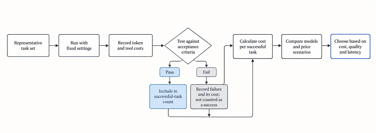
LLM cost per task is the total API spend on every attempt at a set of tasks, divided by the number of attempts that met your acceptance criteria.

The rest of this article is about calculating that number correctly, and about knowing when to trust it.

Key Takeaways
  • Price per token and cost per task can rank models in opposite orders. Kimi K3.1 Pro is half Opus 5.5’s per-token price but cost about 16% more per Artificial Analysis task.
  • Reasoning tokens are billed as output by OpenAI, Anthropic and Google, even when you never see them. Anthropic also bills earlier turns’ thinking as input on its newest models.
  • Caching can swing the bill several-fold. In one public test, a broken cache made a single run cost $17.60 instead of $2.62.
  • Divide by successes, not attempts. Failed runs cost money and produce nothing.
  • Twenty runs can’t separate close results. An 80% and a 65% pass rate from 20 runs each have overlapping confidence intervals.
  • Price changes can settle a close call. One developer test found Gemini 4 Argon roughly level with Opus 5.5 per successful fix. At Argon’s December 1 prices, it would cost about twice as much.

Quick Navigation


The LLM cost per task formula

For one attempt, the API cost is the sum of each token category times its rate, with token counts converted to millions:

Attempt cost = (fresh input tokens  ÷ 1,000,000 × fresh-input rate)
             + (cache-read tokens   ÷ 1,000,000 × cache-read rate)
             + (cache-write tokens  ÷ 1,000,000 × cache-write rate)
             + (billable output     ÷ 1,000,000 × output rate)
             + per-call charges (web search, code containers, grounding)

Then, across a test set:

LLM cost per successful task = sum of all attempt costs ÷ number of successful attempts
LLM cost

Each line has its own billing rules, and they differ by provider. This is the buyer’s cost. What it costs a provider to serve those tokens, and its margin, is a separate question, covered in what inference actually costs per token.

What each line costs at OpenAI, Anthropic and Google
Line itemOpenAI (GPT-5.6 and later)Anthropic (Claude 5.5 models)Google (Gemini 4 Argon)
Fresh inputList rateList rateList rate
Cache read0.1× input; 0.05× on GPT-6.1 Sol and Terra0.1× input; 0.05× on Opus 5.5 and Sonnet 5.5$0.10 per million (0.05× input)
Cache write1.25× input (30-minute) or 2.5× (12-hour)1.25× input (5-minute) or 2× (1-hour)No separate charge listed; caching is implicit only
Reasoning tokensBilled as outputBilled as output, including when thinking text is hiddenBilled as output (“incl. thinking”)
Search tools$10 per 1,000 web searches$10 per 1,000 web searches$14 per 1,000 grounded queries after 5,000 free a month

Sources: OpenAI pricing and prompt caching; Anthropic pricing and prompt caching; Gemini API pricing.

Two details catch people out. Anthropic’s thinking defaults to a display mode of “omitted” on Opus 5.5 and Sonnet 5.5, but its thinking documentation is explicit: “You’re still charged for the full thinking tokens. Omitting reduces latency, not cost.” On those models, previous turns’ thinking blocks also stay in context and are billed as input, so a long agent session pays for old reasoning again on every turn.

Reading usage fields without double-counting

A common error in home-made calculators is adding a field that already contains another one.

  • Anthropic: input_tokens counts only the tokens after the last cache breakpoint. Total input is cache_read_input_tokens + cache_creation_input_tokens + input_tokens, and each part takes its own rate.
  • OpenAI: cached_tokens excludes tokens charged as writes, which appear in cache_write_tokens. Reasoning tokens sit inside output_tokens, under output_tokens_details.reasoning_tokens. Don’t add them again.
  • Truncated responses: with reasoning models, a request that hits its output limit can bill input and reasoning tokens and return no visible answer, as OpenAI’s reasoning guide warns. That attempt still counts toward the cost.

Then reconcile your summed usage against the provider’s invoice for the same period. In July 2026, developers on OpenAI’s forum reported that GPT-5.6 output-token counts were several times higher than the text actually generated. OpenAI didn’t publicly confirm a defect in that thread. Whatever happened there, the invoice is the figure your finance team will pay.

From cost per attempt to LLM cost per successful task

The numerator is everything you paid to get results. That includes failed attempts, automatic retries, intermediate calls inside an agent loop, any model you use as a judge and per-call tool fees. Count each API call once, at the moment it happens. If your harness logs both an agent step and its parent run, sum only one of them.

The denominator is the number of attempts that passed a fixed acceptance test, written before the run. “The tests pass” is a test. “The output looked fine” is not. The same criteria must apply to every model, or the division compares different jobs.

There are two valid ways to define a task:

  • Independent attempts. Each run is scored on its own, which is what most benchmark-style comparisons do.
  • Tasks with a retry policy. A task succeeds if any attempt within, say, three tries passes. Then the cost per task is all spend divided by tasks completed. That matches production better, but pick one definition and use it for every model.

API cost is not the whole bill. Human review, retrieval infrastructure, observability and sandboxes belong in a fully loaded cost per task whenever models differ in how much of that work they create. A model whose failures are obvious and cheap to discard can beat one whose failures look plausible and need a reviewer to catch.

A public test: 20 runs, four models

On 14 October 2026, a developer writing at paddo.dev replayed six merged changes from a production monorepo against four models. Each model got 20 runs (three or four per change) at medium effort in the Claude Code harness. Gemini 4 Argon was routed through OpenRouter. A run passed if the tests that shipped with the original fix passed. Costs were calculated at list prices.

ModelRunsPassing runsTotal costCost per runCost per passing run
Gemini 4 Argon2016$57.68$2.88$3.61
Claude Opus 5.52013$45.81$2.29$3.52
Claude Sonnet 5.52011$11.76$0.59$1.07
GPT-6.1 Sol2011$6.73$0.34$0.61

The totals and pass counts come from the post. The last two columns are our arithmetic, and they check: $57.68 ÷ 16 = $3.605, and $45.81 ÷ 13 = $3.524.

Argon and Opus are close, nine cents apart per passing run. Argon’s per-token prices matched Sonnet 5.5’s at the time ($2 input, $10 output), yet it cost five times as much as Sonnet per run. It wrote 1.37 million output tokens across the 20 runs, 2.8 times as many as Opus.

GPT-6.1 Sol had the lowest cost per passing run, but the post also records five Sol runs that broke a previously passing test, against none for the others. It doesn’t say whether those runs are among Sol’s 11 passes. If “breaks nothing” is part of your acceptance test, Sol’s denominator may shrink, which is why the test has to be written down before anyone divides.

How much a 20-run test can tell you

Not much, at the margin. A 95% Wilson confidence interval on 16 passes out of 20 is about 58% to 92%; for 13 out of 20, about 43% to 82%. The ranges overlap heavily, so a rerun could reverse the order. And six changes from one codebase, with correlated runs on each change, say little about a different stack.

What the December repricing does

Google’s pricing page doubles every Argon token rate on 1 December 2026: input from $2 to $4, cached input from $0.10 to $0.20, output from $10 to $20. If the runs used identical tokens, Argon’s total would become $115.36, or $7.21 per passing run, about twice Opus’s $3.52. We covered the change itself in Gemini 4 Argon pricing doubles Dec 1.

A simple break-even check shows how far the decision moves. One model is cheaper per success than another when its pass rate exceeds the other’s pass rate multiplied by the ratio of their per-attempt costs. Before December, Argon needed a pass rate above 65% × 1.26 ≈ 82% to beat Opus; it scored 80%. After December, it would need 65% × 2.52 ≈ 164%, which is impossible. Even at the bottom of Opus’s confidence interval, Argon would lose. On this test, the price change settles a question the sample size couldn’t.

How caching and reasoning change LLM cost per task

The same post found a stark caching failure. The first Argon run cost $17.60 because it read 8.4 million input tokens and only 59,000 came from cache. The harness inserted system messages that changed the prompt prefix on every call, so Gemini’s implicit cache never matched. After a fix, the same run cost $2.62, with 94% of input served from cache.

The second example is illustrative. The token counts and pass rates are assumptions, not measurements of any real model. Two models attempt the same agent task:

  • Model X: $1 input, $0.05 cache read, $1.25 cache write, $5 output, per million tokens. Pass rate 60%.
  • Model Y: $4 input, $0.20 cache read, $5 cache write, $20 output. Pass rate 85%.
  • Each attempt sends 300,000 input tokens over its turns. When caching works, 270,000 are cache reads and 30,000 are cache writes.
  • Model Y produces 20,000 output tokens per attempt, including reasoning. Model X produces 60,000.
ScenarioCost per attemptPass rateCost per successful task
Model X, cache broken (all 300,000 input tokens fresh)$0.60060%$1.00
Model X, cache working$0.35160%$0.585
Model X, cache working, reasoning doubles to 120,000 output tokens$0.65160%$1.085
Model Y, cache working$0.60485%$0.711

The calculation for the second row: 270,000 × $0.05 + 30,000 × $1.25 + 60,000 × $5, each divided by one million, gives $0.0135 + $0.0375 + $0.30 = $0.351. Dividing by 0.60 gives $0.585.

LLM cost

With caching working, the cheaper model wins. Break the cache, or let it reason twice as long, and the expensive model wins instead. Neither change shows up in a price table.

What published comparisons actually measured

Before using a published cost-per-task figure, check the effort setting, what counted as a task, and whether success was part of the number.

  • Effort settings. Put Gemini 4 Argon’s 36,000 reasoning tokens per task next to Opus 5.5’s 84,000, and Argon looks far leaner. Both figures appear on Artificial Analysis, but they come from different settings: Argon at High effort and Opus 5.5 at Max. At matched High effort, the comparison reverses: Argon used 36,000 reasoning tokens per task to Opus’s 18,000, and 62,000 output tokens in total to Opus’s 36,000. Argon still cost less per task, $1.62 against $1.82, because its tokens were half the price at the time.
  • Vendor claims. OpenAI launched GPT-6.1 Terra on 26 October at $1 input and $5 output. DataCamp’s write-up of the announcement says that at max effort Terra is over three times as token-efficient as Opus 5.5 and a quarter of the price per token, and it puts the combined effect at “9x lower cost per task”, attributed to OpenAI. No benchmark is named, and we couldn’t open OpenAI’s post to check. Three times the efficiency at a quarter of the price would multiply to about 12 times, not 9, so the figure depends on a token breakdown that hasn’t been published. Treat it as a vendor claim to test, not a result.
  • Cost per task is not cost per success. Artificial Analysis computes cost per task from token counts at list prices. It doesn’t divide by how many answers were right. A model that is cheaper per task but scores lower may still cost more per correct answer. As we argued in why benchmark scores don’t transfer to your workload, these numbers are good for building a shortlist, not for making the final decision.

How to measure LLM cost per task on your own workload

  1. Pick 30 to 50 real tasks from production traffic, covering easy, typical and hard cases. More tasks beat more runs of the same task.
  2. Write the acceptance test first: unit tests, a schema check or a fixed-judge rubric, identical for every model.
  3. Fix the configuration: prompts, tools, effort setting, context limits and retry policy.
  4. Log raw usage for every call, including retries and sub-agents, with each token field stored separately.
  5. Price the logs offline against a dated copy of each pricing page, so you can reprice them when rates change.
  6. Check cache hit rates per model. A low rate in a repetitive session usually means the prompt prefix changes between calls.
  7. Reconcile with the invoice for the test window.
  8. Report ranges: pass rate with a confidence interval, cost per attempt, cost per successful task and latency.

Run at least two attempts per task. That shows whether failures are random or the same task fails every time.

A decision rule for LLM cost per task

Compare models on cost per successful task, after deciding what a success is worth. Then apply three checks.

  • If the confidence intervals on pass rate overlap, treat the models as tied on quality and choose on cost per attempt, latency and operational fit.
  • If one model’s cost per attempt is k times another’s, it needs a pass rate more than k times higher to win. When that would take a pass rate above 100%, stop testing.
  • If a success is worth far more than the API cost, as with a merged fix that saves an engineer an hour, pass rate and reviewer time outweigh token prices. Optimise for the fewest failures, then for cost.

Per-token prices still have a job. They tell you where to look first. LLM cost per task tells you what you’ll actually pay.

Frequently asked questions

What is LLM cost per task?

It is the total API spend on all attempts at a set of tasks, divided by the number of attempts that met a fixed acceptance test. Failed attempts, retries, intermediate agent calls and judge-model calls stay in the total, because you paid for them. A broader, fully loaded version adds review time and infrastructure.

How do I calculate LLM API cost for one request?

Multiply each token category by its rate per million tokens: fresh input, cache reads, cache writes and output, including reasoning. Then add per-call tool fees such as web search. Take the counts from the response’s usage object, and check that one field doesn’t already include another before adding them.

Are reasoning tokens billed?

Yes. OpenAI, Anthropic and Google bill reasoning or thinking tokens at the output rate, even when the reasoning text isn’t returned. On Anthropic’s Opus 5.5 and Sonnet 5.5, previous turns’ thinking blocks are also billed as input when they stay in the conversation.

How much does prompt caching save?

Cache reads cost between 5% and 10% of the input rate at OpenAI, Anthropic and Google for current models. OpenAI and Anthropic charge 1.25 times the input rate or more to write to the cache. Savings depend on how much of each request repeats an earlier prefix, so measure the hit rate rather than assuming it.

Is the cheapest model per token ever the cheapest per task?

Often, yes. On Artificial Analysis’s figures, Gemini 4 Argon at High effort cost less per task than Opus 5.5 at High, while its tokens were half the price. The ranking flips when the cheaper model uses many more tokens, misses the cache or fails more often. Only measurement on your own tasks tells you which case you’re in.


Keep reading

AGI vs superintelligence

AGI vs Superintelligence: A New Name Isn’t a New Intelligence

Facts checked against official documents and reporting on 18 November 2026. On 29 September, the White House told federal agencies to stop writing “artificial intelligence” …
AI Coding Agent

AI Coding Agents Are Getting Expensive. Who’s Paying for the Tokens?

Pricing checked on official vendor pages on 17 November 2026. All USD. Cost scenarios are illustrative and labelled as such. On 28 October, TechCrunch published …
Model Weights

Verify Model Weights: 7 Checks Before You Download
Checked against the burner22/numbat repository and its discussions, Hugging Face and PyTorch documentation, and Moonshot AI’s announcement on 2 November 2026. On 1 November, a …
Agentic AI Statistics

30 Agentic AI Statistics for 2026: Adoption, Spending and Risk

Last updated: 15 November 2026. This page is updated monthly; each figure keeps its original publication date. Agent traffic at one healthcare booking platform rose …

Gemini 4 Argon Pricing Doubles Dec 1: What It Costs

Gemini 4 Argon

Last verified: 27 October 2026, against Google’s Gemini API pricing page, Anthropic’s API pricing page and the Artificial Analysis comparison pages linked below.

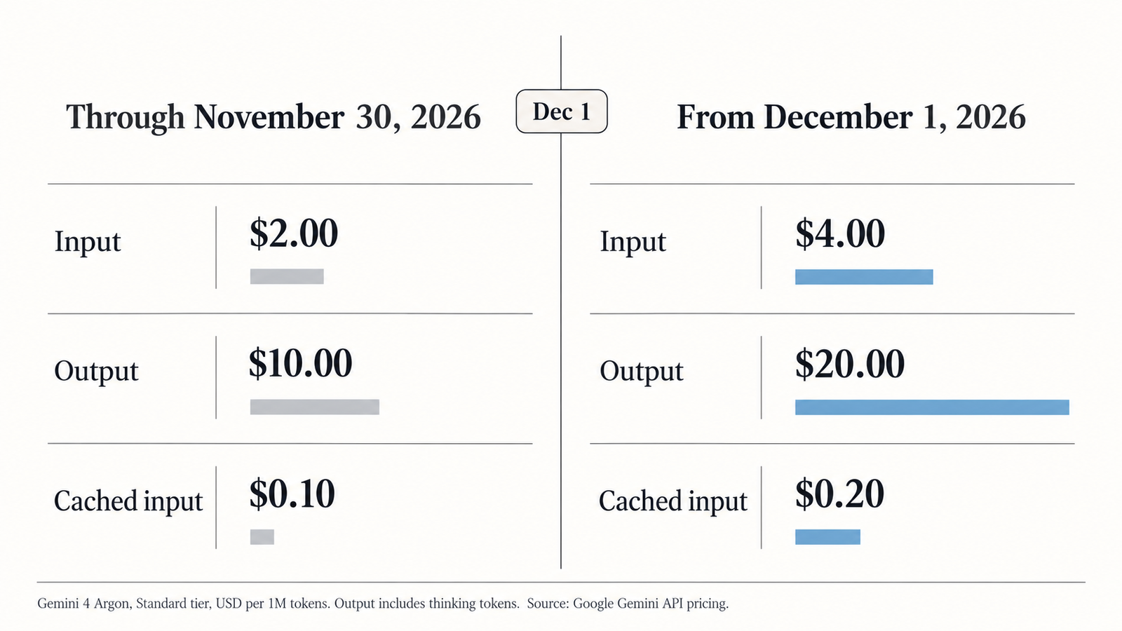
On 1 December 2026, Gemini 4 Argon pricing doubles. Google’s introductory rate of $2 per million input tokens and $10 per million output tokens ends on 30 November, and the standard rate becomes $4 and $20. Cached input goes from $0.10 to $0.20. Those new rates match Claude Opus 5.5’s exactly. Yet the rate card can’t tell you whether Argon stays worth paying for. Argon tends to use more tokens than Opus to finish the same work, and one public coding test found it also finished more of that work. Your bill per completed task depends on both.

That’s what this article works through: what changes, how to cost one task, what the benchmark evidence does and doesn’t show, and how to measure the answer on your own workload before the change lands.

Key Takeaways
  • Every Gemini 4 Argon rate doubles on 1 December 2026: Standard, Batch, Flex and Priority, input, output and cached input. Identical token usage costs exactly twice as much in token charges.
  • From December, Argon’s standard rates equal Claude Opus 5.5’s ($4 input, $20 output, $0.20 cached), so cost differences between them come down entirely to token use.
  • At matched High effort, Artificial Analysis measured Argon using 62,000 output tokens per task against Opus 5.5’s 36,000. At the new prices, that turns Argon’s $1.62 per task into about $3.24, against $1.82 for Opus.
  • In one developer’s coding test, Argon passed 16 of 20 runs against Opus 5.5’s 13. At introductory prices it cost $3.61 per passing run against $3.52; at December prices, about $7.21.
  • Measure cost per successful task on 20 or more of your own tasks before 30 November, then reprice the same token logs at the new rates.

Quick Navigation


Gemini 4 Argon pricing: what changes on December 1?

Google made Argon generally available on 13 October 2026, and its launch post put the end date in a footnote: “After the introductory period expires on November 30, 2026”, the price rises to $4 and $20. The Gemini API pricing page lists both columns for every tier:

Tier (USD per 1M tokens)InputOutput (incl. thinking)Cached input
Standard, through 30 Nov$2.00$10.00$0.10
Standard, from 1 Dec$4.00$20.00$0.20
Batch or Flex, through 30 Nov$1.00$5.00$0.05
Batch or Flex, from 1 Dec$2.00$10.00$0.10
Priority, through 30 Nov$3.60$18.00$0.18
Priority, from 1 Dec$7.20$36.00$0.36
Gemini 4 Argon

Every row doubles. There’s no free tier, and no long-context surcharge is listed for this model. Two lines don’t move: grounding with Google Search and Google Maps stays at $14 per 1,000 requests after 5,000 free a month, with no change shown for December. A workload that leans heavily on grounding will see its total rise by less than 2x.

For comparison, Anthropic’s pricing page lists Claude Opus 5.5 at $4 input, $20 output and $0.20 for cache hits, with Batch at $2 and $10. From December, the two models’ standard token rates are identical. One billing difference remains: Opus charges for writing to its cache ($5 per million for a five-minute cache, $8 for one hour), while Argon’s caching is implicit only, with no write charge listed.

Gemini 4 Argon pricing and the cost of one task

The formula for one request is:

C=Iuncached106Rin+Icached106Rcache+O106RoutC = \frac{I_{uncached}}{10^6} R_{in} + \frac{I_{cached}}{10^6} R_{cache} + \frac{O}{10^6} R_{out}

Here I is input tokens, split into uncached and cached; O is billable output, which for Argon includes thinking tokens, as both the pricing page and Google’s thinking guide state; and R is the rate for each. A task is the sum over every request it makes, including retries and tool-call turns.

Illustrative example, not a measurement. An agent step sends 200,000 input tokens, of which 150,000 hit the cache, and produces 20,000 output tokens, thinking included.

LineThrough 30 NovFrom 1 Dec
50,000 uncached input50,000 ÷ 1M × $2 = $0.100× $4 = $0.200
150,000 cached input150,000 ÷ 1M × $0.10 = $0.015× $0.20 = $0.030
20,000 output20,000 ÷ 1M × $10 = $0.200× $20 = $0.400
Total$0.315$0.630

Same tokens, exactly double the cost. On Claude Opus 5.5 the same token counts would also cost $0.630, plus any cache-write charge to create that cached prefix in the first place.

That’s the controlled, price-only view, and it’s the easy part. The hard part is that two models never use the same tokens for the same job, and Argon’s own usage changes with its thinking level. The evidence on how much it uses is where things get contradictory.

What the benchmark evidence actually shows

Two public sources speak to Argon’s cost per task, and at first glance they disagree.

Artificial Analysis: the configuration matters

Artificial Analysis runs models through its Intelligence Index v4.3.2, a weighted mix of ten evaluations covering agentic knowledge work, coding, scientific reasoning and general knowledge. Its “cost per task” is a weighted average across those evaluations, priced at current list rates using token counts reported by the provider. A “task” here could be a physics problem or a spreadsheet deliverable. It isn’t a software ticket.

The figures widely quoted for Argon (62,000 output tokens and $1.99 per task, against 119,000 tokens and $5.98 for Opus 5.5) are real, but they compare Argon at High thinking against Opus 5.5 at Max effort. Opus at Max scores 58 on the index against Argon’s 53, so that pairing compares a cheaper model with a stronger configuration.

The matched comparison is Argon (High) against Opus 5.5 (High), which score 53 and 54:

Artificial Analysis, read 27 Oct 2026Gemini 4 Argon (High)Claude Opus 5.5 (High)
Intelligence Index v4.3.25354
Output tokens per task62k36k
of which reasoning36k18k
Cost per task, at intro Argon pricing$1.62$1.82
Cost per task, Argon repriced at 1 Dec ratesabout $3.24$1.82

The last row is our calculation: Artificial Analysis’s $1.62 doubled, which holds if token counts and cache-hit rate stay the same. The same Argon (High) entry showed $1.99 per task on the Opus Max page, read the same day; at $1.99, the December figure would be about $3.98. Either way, at matched effort Argon writes 1.7 times as many output tokens as Opus, and at equal rates that costs roughly 1.8 to 2.2 times as much per task.

One developer’s coding test

The second source is a write-up on paddo.dev, published 14 October 2026. Its author replayed six merged changes from one production monorepo on clean snapshots, ran each model 20 times in total through the Claude Code harness at medium effort, and scored each run against the tests the original fix shipped with. Argon ran through OpenRouter.

paddo.dev, 20 runs per modelGemini 4 ArgonClaude Opus 5.5
Runs passing all tests1613
Output tokens1.37M495k
Total cost at list prices$57.68$45.81
Cost per passing run, intro prices$3.61$3.52
Cost per passing run, 1 Dec prices$7.21$3.52

The last two rows are our calculation from the published totals. Two corrections to how this test is often summarised: it’s 20 runs across six changes, not 20 different tasks, and the author doesn’t say whether the totals include retries or tool-call overhead. They also report a proxy fault that broke caching on Argon’s first run, inflating it to $17.60 before a fix brought a comparable run to $2.62. It’s unclear whether that run sits in the total.

One detail in those totals is easy to miss. At list rates, Argon’s output tokens account for about $13.70 of its $57.68, and Opus’s for about $9.90 of $45.81. Most of both bills is input: a coding agent rereads files and context on every turn. Output-token counts alone understate how differently the two models drive a harness.

Why the two sources only seem to disagree

The author contrasts their result with Artificial Analysis showing Argon using fewer tokens than Opus. That contrast comes from the Max-effort pairing. At matched effort, both sources point the same way: Argon generates more tokens than Opus 5.5, 1.7 times as many on Artificial Analysis’s mixed tasks at High and 2.8 times as many on six coding changes at medium.

Where they genuinely differ is quality. Opus scores a point higher on the index; Argon passed three more runs in the coding test, mostly by solving one change (change B) that Opus failed in every run. The author’s own caveat applies: a different codebase puts a different change in that slot. Six changes from one repository are enough for that team’s decision, and not enough to rank the models.

Why Gemini 4 Argon pricing doesn’t tell you the whole bill

The rate card fixes the price of a token. Several things you control, and some you don’t, fix how many tokens you buy.

  • Thinking level. Argon supports low, medium and high thinking, defaults to medium, and bills all thinking tokens at the output rate even though only summaries come back. Artificial Analysis tests at High; the coding test used medium. If your requests don’t need deep reasoning, dropping to low is the single biggest lever after December, and it’s free to test.
  • Cache hits. Argon caches automatically for prompts of at least 4,096 tokens, at 95% off input. The coding test’s proxy fault shows the stakes: the same kind of run cost $17.60 with caching broken and $2.62 with it working, 94% of input served from cache. Anything that changes the start of your prompt between calls (timestamps, reordered tool lists, per-request IDs) quietly turns cheap cached input into full-price input.
  • Retries, tool calls and loops. Every retry and every tool-result turn is another request with its own input bill. An agent that needs three attempts on a hard task pays for all three, which is why cost per successful task is the number that matters.
  • Tier choice. Batch and Flex run at half the standard rate, so from December they cost exactly what Standard costs today. Any work that can tolerate delay, such as evaluations, backfills and nightly jobs, can move tier and stay at the old price. Priority runs at 1.8 times Standard.
  • Time and people. In the coding test, Argon took 991 seconds per run on change B against Opus’s 455. A model that’s cheaper per fix but twice as slow can still cost more if a developer is waiting on it, and a model that fails less can save review time no API bill shows. How inference cost per token is calculated across those layers is covered in our breakdown of the three numbers that matter.

How to measure your own Gemini 4 Argon cost per task

Gemini 4 Argon

You have until 30 November to collect token logs at the cheap rate, and those logs are all you need to price December exactly. The protocol:

  1. Pick 20 to 50 real tasks from your backlog or production traffic. Include a few that are hard.
  2. Freeze everything: instructions, context, tool definitions, model settings (including Argon’s thinking level and the other model’s effort level) and the acceptance test for each task.
  3. Run each model under a documented configuration, in the same harness, from the same region.
  4. Log token counts per request from the API’s usage fields: uncached input, cached input, output and thinking. Keep them per task, not just as a monthly total.
  5. Log every retry, failed run and tool call, plus non-token charges such as search grounding.
  6. Score each run against the same acceptance test. Tests that pass or fail beat a human “looks fine”.
  7. Divide total API cost by successful tasks. Failed runs still count in the numerator.
  8. Record latency and human review time separately, so they can be weighed rather than hidden.
  9. Repeat runs where results vary: three runs per task is a reasonable floor for agentic work.
  10. Reprice the same logs at December rates. For Argon that’s a straight doubling of token charges; nothing else in the calculation changes.

Step 7 is the formula our GPT-6 Sol vs Claude Opus 5.5 comparison uses to fold retries and completion rate into a cost per completed task:

Cost per successful task=∑all runsCrunruns that pass the acceptance test\text{Cost per successful task} = \frac{\sum_{\text{all runs}} C_{\text{run}}}{\text{runs that pass the acceptance test}}

Here’s how the results might look. Every number in this table is illustrative, invented to show the arithmetic. Model X stands for a model priced like Argon, Model Y for one priced like Opus 5.5, including a cache-write charge.

Illustrative, 20 tasksModel X (intro)Model X (from 1 Dec)Model Y
Passing tasks171714
Tokens: uncached / cached / output3.0M / 25M / 1.2Msame2.0M / 15M / 0.5M + 1.0M cache writes
Total API cost$20.50$41.00$26.00
API cost per successful task$1.21$2.41$1.86
Including 15 min review per failure at $60/hour$3.85$5.06$8.29

On API cost alone, December flips this example: X goes from 35% cheaper per success to 30% dearer, and no pass rate out of 20 could save it, since it would need 22 passes to match Y. Add the human cost of failures and X wins at either price. Your own numbers will differ. The structure won’t.

A 20-task run is enough to make an engineering decision for one team on one workload. It isn’t enough to say one model is better in general, and the stochastic spread between runs can be larger than the gap you’re trying to measure.

Should you keep using Gemini 4 Argon after December 1?

It depends on which of these describes you.

  • Argon passes your tests noticeably more often. If failures cost real review or rework time, a higher pass rate can outweigh a doubled token bill, as the illustrative table shows. Re-measure, but don’t switch on price alone.
  • Argon and the alternative pass at similar rates. At equal rates per token, cost tracks token use, and on both public sources Argon uses more. Test the alternative seriously.
  • The work isn’t urgent. Move it to Batch or Flex. From December they cost $2 and $10, exactly today’s Standard rate.
  • You haven’t tuned thinking. Try low thinking on your simpler tasks before comparing models; it may close most of the gap.
  • Latency matters. Argon was the slower model in the coding test, roughly twice as slow on its hardest change. If a person waits on the answer, weigh that alongside cost.
  • Your cache-hit rate is low. Fix prompt prefixes first. The difference between broken and working caching was nearly sevenfold in the one documented run.

There’s no general verdict here, and the evidence doesn’t support one. Artificial Analysis says Argon roughly matches Opus 5.5 at High while writing more. One coding test says it passes more often while writing much more. Both lead to the same practical rule: from 1 December, paying the same rate as Opus only makes sense where Argon’s extra success rate, speed or fit earns back its extra tokens.

Frequently asked questions

When does Gemini 4 Argon pricing increase?

On 1 December 2026. Google’s introductory pricing applies through 30 November 2026, according to its Gemini API pricing page and the footnote to its 13 October launch announcement.

How much will Gemini 4 Argon cost per million tokens from December 1?

On the Standard tier, $4.00 per million input tokens, $20.00 per million output tokens (thinking tokens included) and $0.20 per million cached input tokens. Batch and Flex become $2.00, $10.00 and $0.10; Priority becomes $7.20, $36.00 and $0.36.

Will the price increase double every customer’s API bill?

Token charges double exactly for identical usage, because every Argon rate doubles. Total bills can differ: search grounding fees don’t change, and anyone who lowers thinking levels, improves cache hits, or moves work to Batch or Flex will pay less than double.

Is Gemini 4 Argon still cheaper than Claude Opus 5.5 after December 1?

Not per token: from December both list $4 input, $20 output and $0.20 cached on their standard tiers. Per task, Argon used more output tokens than Opus 5.5 in both public sources checked, so it will often cost more, unless a higher pass rate or lower review time offsets that.

How do you calculate Gemini 4 Argon cost per task?

Add uncached input tokens times $4, cached input times $0.20 and output (including thinking) times $20, each per million tokens, across every request the task makes, retries included. Divide the total over a batch of tasks by the number that passed your acceptance test.

How can developers benchmark the models before the pricing change?

Run 20 to 50 real tasks on each model before 30 November with frozen settings and fixed acceptance tests, logging token counts per request. Then reprice the same logs at December rates. Argon’s charges simply double, so you can compare costs without running anything twice.


Keep reading

AGI vs superintelligence

AGI vs Superintelligence: A New Name Isn’t a New Intelligence

Facts checked against official documents and reporting on 18 November 2026. On 29 September, the White House told federal agencies to stop writing “artificial intelligence” …
AI Coding Agent

AI Coding Agents Are Getting Expensive. Who’s Paying for the Tokens?

Pricing checked on official vendor pages on 17 November 2026. All USD. Cost scenarios are illustrative and labelled as such. On 28 October, TechCrunch published …
Model Weights

Verify Model Weights: 7 Checks Before You Download
Checked against the burner22/numbat repository and its discussions, Hugging Face and PyTorch documentation, and Moonshot AI’s announcement on 2 November 2026. On 1 November, a …
Agentic AI Statistics

30 Agentic AI Statistics for 2026: Adoption, Spending and Risk

Last updated: 15 November 2026. This page is updated monthly; each figure keeps its original publication date. Agent traffic at one healthcare booking platform rose …

Context Engineering: Cost, Latency and Security in AI Agents

context engineering

An agent asked to fix a failing test may make twenty model calls before it answers. The first call carries a system prompt, a few thousand tokens of tool definitions and the user’s request. By the tenth call it is also carrying three file reads, two test runs, a stack trace, a search result and the model’s own earlier reasoning. None of that was written as a prompt, yet all of it shapes the next decision. Context engineering is the work of deciding what goes into each of those calls. As AI applications become stateful, tool-using systems, the wording of the prompt becomes one part of a larger problem: managing context for quality, cost, latency and security all at once.

That last part is the argument of this piece. Most explanations of context engineering treat it as a quality discipline, about getting the right information to the model. It is that, but the same decisions also set the input bill, the time to first token and the set of instructions an attacker can reach. A choice made for one of those reasons changes the other three.

Key Takeaways
  • Context engineering decides the exact tokens in each model call. Prompt wording is one part of it, and in agents often a small one.
  • Agent loops are input-heavy. In the worked example, input was over 90% of the uncached cost, and good cache layout cut the run by about 78%.
  • Prompt order is a cost decision. A volatile value at the top of the prompt can make caching more expensive than not caching.
  • Long context mainly lengthens prefill and time to first token. The size of the effect depends on hardware, serving and cache hits.
  • Everything in context can steer the model. Treat retrieved text, tool outputs and third-party tool descriptions as untrusted, and enforce permissions outside the model.
  • Every context rule should have a test: task success, tokens, cache-read share, latency and injection resistance.

Quick Navigation


The shift from prompt engineering to context engineering

The term is newer than the practice. Anthropic’s Applied AI team, in a September 2025 engineering post titled Effective context engineering for AI agents, described it as “the natural progression of prompt engineering”. It defined context engineering as “the set of strategies for curating and maintaining the optimal set of tokens” during inference. That is a useful working definition, but it is a practitioner’s framing, not a standard. Retrieval-augmented generation, conversation summarisation and tool design all existed before anyone grouped them under one name.

So “replaced” overstates it. Prompt design did not go away; it became one input among several. A well-written system prompt still matters, but in an agent it may be only a few percent of the tokens in a late-stage call. The rest arrives from places the prompt author did not write and often never sees.

DisciplineMain questionTypical artefacts
Prompt engineeringHow should the instructions be worded?System prompt, few-shot examples, output format
Retrieval (RAG)Which external documents are relevant to this query?Index, retriever, reranker, chunks
MemoryWhat from earlier sessions or turns should persist?Notes, summaries, user profiles, vector stores
OrchestrationWhich call happens next, and with which tools?Agent loop, planner, sub-agents, tool router
Context engineeringWhat exact set of tokens enters this call, in what order, and with what trust level?Context assembler, budgets, compaction rules, cache layout

Context engineering sits across the other four. Retrieval decides what might be relevant. Memory decides what might be kept. Context engineering decides what is actually sent, and that decision is made again for every call.

The context budget: what actually enters a model call?

Three numbers are often confused. The context window is the maximum the model will accept. The context budget is what an application chooses to spend, given cost and latency targets. The task requirement is what the call actually needs to succeed. In a healthy system the third is well below the second, and the second well below the first. UniverseBlend’s LLM context window comparison makes the same point from the other side: a model accepting a million tokens “says nothing about how well it uses them”.

A single call in an agent loop typically assembles:

  • System instructions: stable, written by the developer, high trust.
  • Tool definitions: stable within a session. They are often larger than people expect, because every tool brings a name, a description and a JSON schema.
  • Conversation history: grows every turn.
  • Retrieved material: documents, search results and file contents, chosen per query.
  • Tool outputs: API responses, logs and test results, frequently verbose and rarely edited.
  • Summaries and notes: compressed forms of earlier work, written by the model itself.

These components differ in how often they change, how much they cost, and how far they can be trusted. That is why context assembly should be task-specific. A call that decides which file to open needs the file list, not the contents of last week’s design document. A call that writes the final answer may need the reverse.

Anthropic’s post recommends several patterns for keeping the budget under control:

  • Compaction: summarising a conversation as it approaches the limit and starting a fresh window.
  • Tool-result clearing: dropping raw outputs once they have been used.
  • Structured note-taking outside the window.
  • Sub-agents: each works in a clean context and returns a condensed summary.
  • “Just-in-time” retrieval: the agent keeps lightweight identifiers, such as file paths or queries, and loads content only when needed.

Each of these is a decision about what survives into the next call.

The cost of context engineering

Agent loops are input-heavy in a way chat is not, because each call re-sends the accumulated transcript. A worked example makes the size of this visible.

Hypothetical workload. Rates are Anthropic’s published Claude Opus 5.5 prices, checked on 22 October 2026: $4 per million input tokens, $5 per million for 5-minute cache writes, $0.20 per million for cache reads, and $20 per million output tokens.

The agent makes 20 calls. Each carries a 12,000-token stable prefix (system prompt and tool definitions). The transcript grows by 1,500 tokens per call (tool output plus the model’s reply). Each call generates 500 output tokens. Across the run, that is 525,000 input tokens and 10,000 output tokens, and the last call alone sends 40,500 input tokens.

StrategyWhat is billedTotal
No caching525,000 input × $4 + 10,000 output × $20$2.30
Cache the stable prefix only12,000 written once, 228,000 read, 285,000 uncached history, output$1.45
Cache the growing prefix each turn40,500 written, 484,500 read, output$0.50
Prefix broken on every call (e.g. a timestamp at the top)525,000 written at $5, output$2.83
context engineering

Three things stand out. Input is $2.10 of the $2.30 uncached total, so here context, not generation, is the bill. Caching the whole growing prefix cuts the run cost by about 78%. And a single volatile value placed early in the prompt makes caching cost more than not caching, because every call pays the write premium and none of them get a read.

That last row is the context-engineering lesson. Anthropic’s prompt-caching documentation says cache hits “require 100 percent identical prompt segments” and that prefixes are built in the order tools, system, then messages. OpenAI’s prompt-caching guide tells developers to keep stable content first and dynamic content last, and to move timestamps and user-specific values later. On both platforms, cache economics depend on where things sit in the prompt, not just on how much there is.

Caching also has limits worth stating. Anthropic’s default cache lives five minutes (refreshed on use), so a tool call that runs longer than that lets the prefix expire. Opus 5.5 will not cache prompts under 512 tokens, and OpenAI’s minimum on GPT-5.6 and later is 1,024. On Anthropic’s API, changing a tool definition invalidates the entire cache. The worked example assumes none of these interruptions happen, and a real run will do worse.

The latency tax of context engineering

Inference has two phases. In prefill, the model processes every input token, largely in parallel, and builds the key-value (KV) cache that generation will read from. In decode, it produces output one token at a time. The Splitwise paper from Microsoft researchers calls these “a compute-intensive prompt computation” and “a memory-intensive token generation”. The DistServe authors tie time to first token (TTFT) to prefill, and time per output token to decode.

Long context therefore lands mainly on TTFT. A 40,500-token prompt has far more prefill work than a 12,000-token one, and that work happens before the user sees anything. The relationship is not a fixed per-token cost, though. It depends on the attention implementation, the hardware, how the provider batches requests, queueing at the moment of the call and, above all, cache hits. Both major providers say caching reduces time spent processing input. Anthropic says users “generally see improved time-to-first-token for long documents”. Neither publishes a universal figure, and this article does not invent one. UniverseBlend’s LLM inference latency measurements show how far TTFT varies by provider even before prompt length is considered.

For agents, the model’s prefill time is only part of the wait. End-to-end latency adds network round trips, retrieval queries, tool execution and orchestration logic, multiplied by the number of steps. Trimming context helps the inference share of that. It does nothing for a slow database query or a test suite that takes four minutes. A latency budget for an agent should be measured per component before anyone decides to cut context to fix it.

Context engineering is also a security boundary

Everything in a model’s context can influence its next action. That is how the model is designed to work, and it is also the security problem. Greshake and colleagues’ 2023 paper on indirect prompt injection put it plainly: “LLM-Integrated Applications blur the line between data and instructions”. An attacker who cannot reach the prompt can still plant text in a web page, a document or a code comment that the application is likely to retrieve.

OWASP’s LLM01:2025 Prompt Injection entry separates direct injection from indirect injection, “when an LLM accepts input from external sources, such as websites or files”. It also notes that RAG and fine-tuning “do not fully mitigate” the risk. Agents widen the set of sources: retrieved documents, tool outputs that talk back, earlier conversation turns, and tool descriptions themselves. The Model Context Protocol specification says “descriptions of tool behavior such as annotations should be considered untrusted, unless obtained from a trusted server”. It also states that “MCP itself cannot enforce these security principles at the protocol level.” UniverseBlend’s eight classes of prompt injection maps how each of these entry points behaves.

context engineering

An illustrative scenario, not a reported incident: a support agent can read tickets and issue refunds through a tool. A customer submits a ticket whose body contains text formatted like a system note telling the assistant to refund the order in full and close the ticket. The ticket enters the context as retrieved material. Whether the model follows it depends on the model, the prompt and the formatting. Context engineering can lower the odds: mark the ticket body as untrusted data, keep it in a delimited block, and avoid putting it near the instructions. None of that is a guarantee. OpenAI’s research on an instruction hierarchy reports that training models to prioritise privileged instructions substantially improves robustness. That lowers the risk; it doesn’t remove it.

The control that actually holds sits outside the context. The refund tool should check, on the server, that the caller is authorised to refund that order, that the amount is under a limit, and that refunds above the limit need human approval. OWASP’s mitigations say the same: least privilege, functions handled in code rather than by the model, and “human-in-the-loop controls for privileged operations”. The distinction to keep is between what the model sees and what the application lets it do. Context filtering reduces exposure. Authorisation, input validation on tool arguments, sandboxing and approval gates decide the damage.

A context engineering architecture that can be tested

Treating context as an engineered component means every assembly rule should have a measurement attached. A practical architecture has five parts:

  • An assembler that builds each call from typed components (instructions, tools, history, retrieved items, tool outputs), each tagged with its source and trust level.
  • A budget per call type, set in tokens. Compaction or retrieval triggers when the budget is reached, not when the model’s limit is.
  • A cache layout: stable components first, in a fixed order, with volatile values pushed to the end.
  • A retrieval policy that prefers identifiers and on-demand loading over pre-stuffing.
  • An enforcement layer for tool calls, independent of anything in the context.
DecisionWhat to measureHow
What stays in the active contextTask success rate vs tokens per callRun the same eval set with and without each component
What is retrieved on demandRetrieval precision and recall; task successLabelled queries with known relevant documents
What is summarisedAccuracy of facts carried across compactionProbe questions about pre-compaction details
What is removedSuccess rate and tokens after clearing tool outputsAblation on long-running tasks
What is cachedCache-read share of input tokens; cost per taskProvider usage fields per request
What is treated as untrustedInjection success rateSeeded malicious documents and tool outputs in a red-team suite
What needs independent enforcementUnauthorised actions attempted vs executedServer-side logs of denied tool calls

The cache row is the easiest to start with, because both major providers report cached tokens in the response usage data. The security row is the one most often skipped. An agent that has never been tested against a poisoned document hasn’t shown that its context handling is safe.

When more context is the wrong answer

Long windows invite a simple strategy: include everything and let the model sort it out. The evidence says that is not free. The Lost in the Middle study (Liu et al., TACL) found that performance was “often highest when relevant information occurs at the beginning or end of the input context” and dropped when the relevant facts sat in the middle. Chroma’s Context Rot report, testing 18 models in July 2025, found that performance “grows increasingly unreliable as input length grows” and that “even a single distractor reduces performance”. The authors are clear that their evaluation is “not exhaustive of real-world use cases” and that they do not explain the mechanism. These are measured tendencies on specific tasks, not a law that every extra token makes every model worse.

In practice, more context goes wrong in a few recognisable ways:

  • Stale information (an earlier file version, a superseded plan) competes with current facts.
  • Duplicated evidence inflates the apparent weight of one source.
  • Conflicting sources force the model to arbitrate without being told which source is authoritative.
  • Summaries can be wrong. A compaction that drops a constraint will mislead every later call, and nothing in the context will flag it.
  • Unedited tool output buries a single error line in kilobytes of log.

A larger window still earns its place for some work: reasoning across a whole contract, comparing two long documents, or a codebase question whose answer is spread across many files. The case for it is strongest when the task genuinely needs the whole input and weakest when the window is used as a substitute for retrieval. Selective retrieval and a smaller context usually win on cost, latency and attack surface together. The burden of proof belongs on the larger context, and an eval on your own tasks is where that proof should come from.

References and further reading

  1. Effective context engineering for AI agents. Anthropic Applied AI team (Rajasekaran, Dixon, Ryan, Hadfield et al.), 29 Sep 2025. https://www.anthropic.com/engineering/effective-context-engineering-for-ai-agents. Vendor engineering guidance: the definition, compaction, note-taking, sub-agents and just-in-time retrieval.
  2. Lost in the Middle: How Language Models Use Long Contexts. Liu, Lin, Hewitt, Paranjape, Bevilacqua, Petroni, Liang. TACL; arXiv v1 6 Jul 2023. https://arxiv.org/abs/2307.03172. Research: position effects in long contexts.
  3. Context Rot: How Increasing Input Tokens Impacts LLM Performance. Hong, Troynikov, Huber (Chroma), 14 Jul 2025. https://www.trychroma.com/research/context-rot. Vendor research report: reliability declines with input length; distractor effects; stated limitations.
  4. Not what you’ve signed up for: Compromising Real-World LLM-Integrated Applications with Indirect Prompt Injection. Greshake, Abdelnabi, Mishra, Endres, Holz, Fritz. arXiv, Feb 2023 (v2 May 2023). https://arxiv.org/abs/2302.12173. Research: indirect prompt injection.
  5. LLM01:2025 Prompt Injection. OWASP Gen AI Security Project. https://genai.owasp.org/llmrisk/llm01-prompt-injection/. Industry guidance: direct vs indirect injection; RAG and fine-tuning don’t fully mitigate it; least privilege; human approval.
  6. The Instruction Hierarchy: Training LLMs to Prioritize Privileged Instructions. Wallace, Xiao, Leike, Weng, Heidecke, Beutel (OpenAI), arXiv, 19 Apr 2024. https://arxiv.org/abs/2404.13208. Research: training-based robustness to injection.
  7. Model Context Protocol Specification (schema 2026-07-28), Security and Trust & Safety section. https://modelcontextprotocol.io/specification/latest. Official spec: untrusted tool descriptions; the protocol cannot enforce its security principles.
  8. Prompt caching. Anthropic (Claude API docs). https://platform.claude.com/docs/en/build-with-claude/prompt-caching. Official docs: exact-match requirement; tools → system → messages order; 5-minute default TTL; 512-token minimum; TTFT improvement.
  9. Pricing. Anthropic (Claude API docs). https://platform.claude.com/docs/en/about-claude/pricing. Official docs: Opus 5.5 rates used in the worked example.
  10. Prompt caching. OpenAI (API docs). https://developers.openai.com/api/docs/guides/prompt-caching. Official docs: static-first ordering; full-prefix match; 1,024-token minimum; “up to 95%” discount.
  11. Splitwise: Efficient generative LLM inference using phase splitting. Patel, Choukse, Zhang, Shah, Goiri, Maleki, Bianchini (Microsoft), arXiv, 30 Nov 2023. https://arxiv.org/abs/2311.18677. Research: prefill is compute-intensive and decode memory-intensive.
  12. DistServe: Disaggregating Prefill and Decoding for Goodput-optimized LLM Serving. Zhong et al., arXiv, 18 Jan 2024. https://arxiv.org/abs/2401.09670. Research: TTFT tied to prefill; TPOT tied to decode.

Frequently Asked Questions

What is context engineering in AI?

Context engineering is the practice of deciding exactly what information enters each model call: instructions, history, retrieved documents, tool definitions, tool outputs and summaries, along with their order and trust level. It matters most in multi-step agents, where the context is rebuilt for every call.

How is context engineering different from prompt engineering?

Prompt engineering focuses on how instructions are written. Context engineering includes that, but also manages everything else the model sees, much of which the developer never writes directly, such as search results and tool outputs.

Is RAG a form of context engineering?

RAG is one technique within it. Retrieval decides which documents might be relevant. Context engineering also decides how many of them to include, where to place them, whether to summarise them and how far to trust them.

How does context engineering reduce LLM costs?

It reduces costs by sending fewer unnecessary tokens and by ordering prompts so that stable content can be served from cache at a fraction of the input price. Savings depend on the provider’s cache rules, minimum lengths, cache lifetimes and write charges. Caching is not automatically cheaper.

How does context engineering improve AI agent security?

It limits and labels untrusted content, which reduces the chance that injected instructions steer the model. It does not prevent prompt injection on its own. Tool permissions, argument validation, sandboxing and human approval have to be enforced outside the model.

What tools or techniques are used for context engineering?

Common techniques include retrieval with reranking, compaction or summarisation, clearing tool results, structured notes stored outside the window, sub-agents with isolated contexts, cache-aware prompt ordering, and per-call token budgets. The tooling varies; the techniques are what carry over.


Keep reading

AGI vs superintelligence

AGI vs Superintelligence: A New Name Isn’t a New Intelligence

Facts checked against official documents and reporting on 18 November 2026. On 29 September, the White House told federal agencies to stop writing “artificial intelligence” …
AI Coding Agent

AI Coding Agents Are Getting Expensive. Who’s Paying for the Tokens?

Pricing checked on official vendor pages on 17 November 2026. All USD. Cost scenarios are illustrative and labelled as such. On 28 October, TechCrunch published …
Model Weights

Verify Model Weights: 7 Checks Before You Download

Checked against the burner22/numbat repository and its discussions, Hugging Face and PyTorch documentation, and Moonshot AI’s announcement on 2 November 2026. On 1 November, a …
Agentic AI Statistics

30 Agentic AI Statistics for 2026: Adoption, Spending and Risk

Last updated: 15 November 2026. This page is updated monthly; each figure keeps its original publication date. Agent traffic at one healthcare booking platform rose …

AI API Pricing 2026: Every Model, Input and Output

AI API pricing comparison

On the official price lists, GPT-6.1 Sol costs half as much per token as Claude Opus 5.5: $2 against $4 per million input tokens, and $10 against $20 for output. Send each model one 300,000-token prompt that returns a 2,000-token answer, though, and the bills come out at $1.23 and $1.24. OpenAI doubles the input rate once a prompt passes 272,000 tokens. Anthropic charges Opus 5.5 the same rate across its whole 1M-token window. The headline ratio says 2:1. For that request, the real ratio is close to 1:1.

That gap between the published rate and the invoice is the subject of this guide. The tables below give the verified rates. The rest of the guide covers the rules that decide what you actually pay.

Key Takeaways
  • Output tokens usually decide the bill. In the worked example below, output is 2 million of 22 million tokens but makes up roughly half of the cost before caching and nearly all of what remains after it.
  • Cache reads cost 2% to 10% of the ordinary input rate, depending on provider and model. Caching discounts only the input side, so in the worked example a 98% hit rate on the cache-eligible tokens cuts the bill by about 31%, not 90%.
  • Cache writes are a separate line item at OpenAI (1.25× input for 30 minutes) and Anthropic (1.25× for 5 minutes, 2× for one hour). DeepSeek and Google bill caching differently, so cached rates are not like-for-like across providers.
  • Long-context thresholds can reprice a whole request. OpenAI’s GPT-6 models double input and cache rates above 272K input tokens. Gemini 3.1 Pro Preview reprices above 200K. Opus 5.5 has no long-context tier.
  • Three of the requested names do not match a documented, priced API model: Qwen 4, a current first-party Llama API price, and an official Kimi K3 price we could read directly. Details are in the status table.
  • Gemini 3.6 Flash prices double on 1 January 2027, according to Google’s pricing page. Any budget that runs into next year needs both rates.

Quick Navigation


AI API pricing comparison: the October 2026 snapshot

AI API pricing comparison

All prices below are in US dollars per one million tokens, for the standard (real-time) service tier, as published on each provider’s official pricing page and checked on 22 October 2026. Providers did not all change prices on that date; it is simply the date we checked. The table is split in two so it stays readable on a phone. Table 1 gives the token rates, and Table 2 gives the conditions that change them.

Table 1. Token rates (USD per 1M tokens, standard tier, verified 22 Oct 2026)

ProviderModel / API IDInputOutputCached inputCache writes
OpenAIGPT-6.1 Sol gpt-6.1-sol$2.00$10.00$0.10$2.50 (30-min TTL); $5.00 (12-h TTL)
OpenAIGPT-6 Sol gpt-6-sol$2.00$10.00$0.20$2.50
OpenAIGPT-6 Luna gpt-6-luna$0.10$0.50$0.01$0.125 (30-min); $0.25 (12-h)
AnthropicClaude Opus 5.5$4.00$20.00$0.20$5.00 (5-min); $8.00 (1-h)
AnthropicClaude Sonnet 5.5$2.00$10.00$0.10$2.50 (5-min); $4.00 (1-h)
GoogleGemini 3.1 Pro Preview gemini-3.1-pro-preview$2.00$12.00$0.20Storage: $4.50 per 1M tokens per hour
GoogleGemini 3.6 Flash gemini-3.6-flash$0.75$3.75$0.075Storage: $0.50 per 1M tokens per hour
MistralMistral Large 4 mistral-large-4$1.36$4.18$0.14Not published
DeepSeekdeepseek-v4-pro (V4-Pro-0813)$1.32$3.96$0.044Not applicable (misses billed as input)
DeepSeekdeepseek-flash (V4.1-Flash-1017)$0.30$1.20$0.006Not applicable (misses billed as input)
Alibaba CloudQwen3.8-Max qwen3.8-max$2.00$6.00See pricing conditionsNot published
MiniMaxMiniMax-M3.1-Flash$0.15$0.60$0.015Not published
Moonshot AIKimi K3 kimi-k3$3.00*$15.00*$0.30*Not verified

Kimi K3 figures are from Together AI’s serverless price list, a third-party host. Moonshot’s own price table did not render for verification. DeepSeek rates are peak-hour rates; off-peak rates are half.

Table 2. Conditions that change the rate

ModelLong-context tierBatch discountPricing condition
GPT-6.1 Sol, GPT-6 Sol, GPT-6 LunaAbove 272K input tokens: 2× input and cache rates, 1.5× output, for the whole request50% (Batch and Flex)Fast mode 2×; regional processing +10%
Claude Opus 5.5, Sonnet 5.5None; full 1M window at standard rates50%US-only inference 1.1×; Opus 5.5 Fast mode $8 / $40
Gemini 3.1 Pro PreviewAbove 200K: $4.00 input, $18.00 output, $0.40 cache50%Preview model
Gemini 3.6 FlashNone listed50%From 1 Jan 2027: $1.50 / $7.50 / $0.15 cache
Mistral Large 4Not publishedNot published for this modelPublic Preview (v26.10)
DeepSeek V4 Pro and FlashNone; 1M contextNot publishedOff-peak 50% off; peak is 01:00–04:00 and 06:00–10:00 UTC on weekdays
Qwen3.8-MaxSingle tier, 0–1MNot labelledBatch and cache discounts cannot be combined
MiniMax-M3.1-FlashNot publishedNot publishedNo effective date shown
Kimi K3No context-length tiering (official quickstart)Not verifiedCache writes billed by 5-min or 1-h TTL; rates not verified

Table labels. Not published: the provider’s official page gives no figure. Not applicable: the provider’s billing model has no such charge. Not verified: a figure exists but we could not confirm it on an official page. See pricing conditions: the rate depends on a rule described elsewhere. A missing cache price never means free caching.

Which requested models could be verified

This article started from a list of model names. Not all of them match a documented API product.

Requested nameStatusWhat we found
GPT-6 SolVerified current modelStill priced on its own model page, but GPT-6.1 Sol is newer and has cheaper cache reads
GPT-6 LunaVerified current modelPriced as listed above
Opus 5.5Verified current modelClaude Opus 5.5, priced as listed above
Gemini 3.1 ProVerified, previewAPI ID gemini-3.1-pro-preview
Gemini 3.6 FlashVerified current modelRates double on 1 Jan 2027; Gemini 3.8 Flash has the same rates
LlamaNo first-party API price locatedLlama 4 (April 2025) is the latest Llama release; Meta’s newest open-weight model is Muse Spark Open
Qwen 4Name could not be verifiedAlibaba’s newest documented models are Qwen3.8-Max and Qwen3.8 Flash
Mistral Large 4Verified, Public PreviewReleased 6 October 2026
MiniMax M3.1 FlashVerified current model$0.15 / $0.60 is correct, in USD per 1M tokens
DeepSeekVerified current modelsTwo models, with peak and off-peak pricing
KimiVerified model; price unconfirmed at sourcekimi-k3 is current; the official price table did not render

Two corrections are worth stating plainly. No Alibaba documentation we found describes a “Qwen 4”, so this article prices Qwen3.8-Max instead and labels it as Qwen3.8-Max. On Mistral, the marketing pricing page still says “Mistral Large costs $0.5 /M tokens in and $1.5 /M tokens out”. The developer documentation shows that rate belongs to Mistral Large 3. Large 4 lists at $1.36 and $4.18.

The cost behind the headline rate

A pricing page lists up to six token categories, and a real request can touch all of them.

  • Ordinary input is every prompt token that the provider processes from scratch: the system prompt, tool definitions, retrieved documents, conversation history and the user’s message.
  • Output covers every token the model generates. On reasoning models that includes hidden thinking tokens. Google says this directly: Gemini output prices include thinking tokens. A model that thinks for 4,000 tokens before writing a 300-token answer bills 4,300 output tokens.
  • Cached input is prompt content the provider has already processed and stored, so it is billed at a reduced read rate.
  • Cache writes are the cost of storing that prefix the first time. OpenAI and Anthropic charge a premium for this. Google instead charges hourly storage on explicit caches.
  • Long-context tiers reprice a request once its prompt passes a threshold. OpenAI applies the higher rate to the entire request, not just the tokens above the line.
  • Batch pricing takes 50% off at OpenAI, Anthropic and Google in exchange for asynchronous processing. It suits evaluations, backfills and document processing. It doesn’t suit anything a user is waiting on.

The headline input and output pair is therefore the lowest price a request can reach, with no conditions applied. Most real workloads pay for at least two of the other four categories.

Cached-input pricing in practice

Prompt caching stores the processed form of a repeated prompt prefix, so the provider can skip recomputing it on the next request. The provider passes part of that saving back as a lower rate on the tokens that hit the cache. The mechanism differs enough between providers that a cached rate on one page is not directly comparable with a cached rate on another.

Anthropic’s prompt-caching documentation uses explicit breakpoints, with up to four per request. The minimum cacheable prompt for Opus 5.5 is 512 tokens. The default cache lives for five minutes and is refreshed at no cost each time it is used. A 5-minute write costs 1.25× the base input rate and a 1-hour write costs 2×. Reads cost 0.1× on most models, but 0.05× on Opus 5.5 and Sonnet 5.5. Changing a tool definition invalidates the whole cache.

OpenAI’s prompt-caching guide says GPT-5.6 and later support both implicit and explicit caching. The minimum is 1,024 tokens. The default lifetime is at least 30 minutes, and a 12-hour option is available in the Responses API. Writes cost 1.25× ordinary input for the 30-minute lifetime and 2.5× for 12 hours. Reads cost 0.1×, or 0.05× on GPT-6.1 Sol. The guide adds that “cache-write pricing is not an additive fee”: each input token is billed at exactly one rate.

Google’s context-caching documentation says implicit caching is on by default for Gemini 2.5 and newer, with a 4,096-token minimum on Gemini 3.1 Pro Preview and 3.6 Flash. Explicit caches add hourly storage charges, listed on the pricing page.

DeepSeek lists only two input rates, cache hit and cache miss. A cache miss is simply the ordinary input rate.

Three practical consequences follow:

  1. A cache hit is not guaranteed. The prefix has to match exactly. Any change to a timestamp, a tool list or a thinking setting early in the prompt breaks it.
  2. Writes cost money only at some providers. At Anthropic, a 1-hour cache write costs 2× input. The prefix must then be read at least twice before the write pays for itself.
  3. A cheaper read rate does not guarantee a cheaper bill. It does nothing to output, and it does nothing if your traffic pattern lets the cache expire between requests.

A worked example: 22 million tokens, with and without caching

This example is hypothetical. The workload is invented to show the mechanics. The rates are Anthropic’s official Opus 5.5 rates as listed on 22 October 2026.

Workload

  • 10,000,000 ordinary input tokens (user messages and retrieved documents that change on every request).
  • 10,000,000 cache-eligible input tokens: a 50,000-token shared prefix (system prompt, tool definitions and a reference document) sent with 200 requests.
  • 2,000,000 output tokens.

Assumption about cache creation. Traffic gaps let the 5-minute cache expire four times, so the prefix is written four times: 4 × 50,000 = 200,000 write tokens. The remaining 9,800,000 cache-eligible tokens are reads.

Rates (Opus 5.5, USD per 1M tokens): input $4.00; 5-minute cache write $5.00; cache read $0.20; output $20.00.

Formula: Total = (ordinary input × input rate) + (cache writes × write rate) + (cache reads × read rate) + (output × output rate), with each token count divided by 1,000,000.

LineTokensRateCost
Ordinary input10,000,000$4.00$40.00
Cache writes (5-min)200,000$5.00$1.00
Cache reads9,800,000$0.20$1.96
Output2,000,000$20.00$40.00
Total with caching$82.96
Total without caching (20M input at $4)$120.00
AI API pricing comparison

Caching saves $37.04, or 30.9%. On the cached tokens alone, the effective rate falls from $4.00 to about $0.30 per million (writes plus reads, divided by 10 million). The total bill falls by less than a third, because ordinary input and output make up $80 of what remains, and caching touches neither.

The same workload on GPT-6.1 Sol, at $2.00 input, $2.50 write, $0.10 read and $10.00 output, costs $41.48 with caching against $60.00 without. That is the same 30.9% saving, because OpenAI’s write and read multipliers for this model happen to mirror Anthropic’s. Switching to 1-hour Anthropic writes ($8.00) raises the Opus total to $83.56. That costs more here, but it would cost less if longer gaps between requests were forcing extra rewrites.

When a cheaper model costs more

The opening example has a sharper version. GPT-6.1 Sol, with a 270,000-token prompt and a 2,000-token answer:

  • 270,000 × $2.00 + 2,000 × $10.00 = $0.56

Add 10,000 tokens to that prompt, taking it to 280,000:

  • 280,000 × $4.00 + 2,000 × $15.00 = $1.15

A 3.7% longer prompt roughly doubles the cost, because the long-context rate applies to the whole request. At 300,000 tokens, GPT-6.1 Sol ($1.23), Gemini 3.1 Pro Preview ($1.24 at its above-200K rates) and Opus 5.5 ($1.24) all land within about a cent of each other. In that band, a choice between them should rest on output quality and latency rather than price.

The second trap is costing a single call instead of a successful task. Cost per success = cost per attempt ÷ success rate. Hypothetical example: a pipeline step sends 20,000 input tokens and receives 3,000 output tokens. On MiniMax-M3.1-Flash ($0.15 / $0.60) one attempt costs $0.0048; on Opus 5.5 ($4 / $20) it costs $0.10. Even if the small model succeeds half the time and Opus 5.5 nine times in ten, the token cost per success is about $0.01 against $0.11. On tokens alone, the cheaper model still wins.

What flips the comparison is what a failure sets off: a human review, a rolled-back change, a customer ticket. If each failure costs $2 of someone’s time, the expected cost per attempt becomes about $1.00 for the small model and $0.30 for Opus 5.5. These success rates are invented for illustration. Measure your own before treating any per-token figure as the cost of the work.

Hosted API versus open-weight deployment

Several models in the table publish their weights: Mistral Large 4 (weights promised), Kimi K3, Qwen3.8-Max (released openly as Qwen3.8-2.4T-A95B) and Meta’s Muse Spark Open. That makes them available to self-host. It doesn’t make them free.

The hosted rates above are directly comparable with each other. Self-hosted costs are not comparable with them on a per-token basis until you supply your own figures for:

  • GPU rental or ownership cost per hour, and how many GPUs the model needs at your chosen quantization.
  • Achieved throughput in tokens per second at your real batch size and input/output mix.
  • KV-cache memory for your context lengths, which caps concurrency.
  • Utilisation: an accelerator that sits idle 80% of the time costs five times more per token than one at full load.
  • Engineering, orchestration, monitoring, storage and on-call time.

UniverseBlend’s breakdown of self-hosted LLM cost and its five hidden fees works through these layers with stated assumptions. For current accelerator rates, see our GPU cloud pricing 2026 guide. We do not quote a universal self-hosted price per million tokens, because no honest one exists.

Third-party hosts sit between the two. Together AI lists Llama 3.3 70B at $1.04 per million tokens for both input and output, and DeepSeek V4 Pro at the same $1.32 and $3.96 DeepSeek charges at peak. Hosted open-weight prices can match or exceed the original lab’s API, so check both.

A practical API cost-estimation method

  1. Log a representative day of traffic and count tokens per request in four buckets: stable prefix, variable input, visible output and reasoning output.
  2. Find the prefix share. If 40% or more of input tokens repeat across requests within the cache lifetime, caching is worth engineering for.
  3. Estimate the hit rate honestly. Count how often gaps between requests exceed the cache lifetime (5 minutes, 30 minutes or 1 hour, depending on provider and setting). Each gap means another write.
  4. Check every threshold. Record your 95th-percentile prompt length and compare it against 200K (Gemini 3.1 Pro), 272K (GPT-6 family), 256K (several Qwen3.x Plus and Flash models) and 512K (MiniMax-M3).
  5. Apply the formula for each candidate model and multiply by monthly volume.
  6. Move what can wait to batch. Anything that can tolerate hours of delay usually gets 50% off.
  7. Add a margin for retries and failed requests. Our analysis of AI API rate limits in 2026 explains why failed calls still consume capacity.

What changes the bill

  • OpenAI: whole-request repricing above 272K input tokens; cache writes at 1.25× (30 minutes) or 2.5× (12 hours); Fast mode at 2×; regional processing at +10% for models released on or after 5 March 2026.
  • Anthropic: no long-context surcharge on Opus 5.5; a 512-token cache minimum; US-only inference at 1.1×.
  • Google: the above-200K tier on Gemini 3.1 Pro Preview; Flash prices doubling on 1 January 2027; hourly storage for explicit caches.
  • DeepSeek: time-of-day pricing, with weekday peak windows at double the off-peak rate.
  • Alibaba Model Studio: tiered input pricing on many Qwen Plus and Flash models; batch and cache discounts that cannot be stacked.
  • MiniMax: M3 pricing that changes above 512K input tokens; a Priority tier at 1.5×.

Conclusion

Pick the model on quality for your task first. Then let cost choose between the models that pass. Within that shortlist:

  • Output-heavy work (long generation, agents that write code): compare output rates first.
  • Prefix-heavy work (support bots, RAG with a fixed corpus, agents with long tool lists): compare cache read and write rates, and check whether your traffic keeps the cache warm.
  • Long-document work above 200K tokens: the threshold matters more than the headline rate.
  • Offline work: price it at batch rates.

Recheck the rates before you commit a budget. Three of the prices in this article carry a known end date, a preview label or a pending change.

Frequently asked questions

Which AI API is cheapest for input tokens?

Among the models checked on 22 October 2026, GPT-6 Luna has the lowest standard input rate, at $0.10 per million tokens. DeepSeek’s deepseek-flash drops to $0.15 off-peak, and MiniMax-M3.1-Flash is $0.15. These are small models, though, and not substitutes for frontier models on hard tasks.

Which AI API is cheapest for output tokens?

GPT-6 Luna, at $0.50 per million output tokens. Among the larger models, DeepSeek V4 Pro ($3.96 at peak, $1.98 off-peak) and Mistral Large 4 ($4.18) cost well below Opus 5.5 ($20) and Gemini 3.1 Pro Preview ($12).

Which providers offer cached-input pricing?

All of the providers verified here publish a cached-input rate except Alibaba, which points to a separate caching page instead of listing a per-model figure. Cache-write charges and eligibility rules differ by provider.

How much can prompt caching save?

The read discount is roughly 90% to 98% on cached tokens, depending on the model. On a whole bill, the saving depends on how much of the input is a repeated prefix and how much of the cost is output. In our worked example it was about 31%.

Does batch processing reduce API costs?

Yes. OpenAI, Anthropic and Google each publish 50% off for asynchronous batch jobs. The other providers’ batch discounts could not be verified per model.

Why does long-context pricing sometimes increase?

Longer prompts need more compute and memory per request, and some providers price that in with a threshold. OpenAI applies its higher rate to the entire request once the prompt passes 272K input tokens.

Are open-weight models cheaper than hosted APIs?

Only at sustained, high utilisation with engineering capacity to spare. The weights are free to download, but running them means paying for hardware, operations and idle capacity.

How should a startup estimate its monthly API bill?

Measure real token counts per request, split them into prefix, variable input and output, apply each candidate model’s formula, and then add 10% to 20% for retries. Recheck after the first month of production traffic.

How often should AI API prices be rechecked?

Monthly at minimum, and before any budget commitment. This snapshot already contains a scheduled price change (Gemini Flash) and two preview-labelled models.

How these prices were checked. Every rate in Tables 1 and 2 was read from the provider’s official pricing or model page on 22 October 2026, except the Kimi K3 rates, which are labelled as third-party. Totals and derived long-context rates are our own calculations from those published rules.


Keep reading

AGI vs superintelligence

AGI vs Superintelligence: A New Name Isn’t a New Intelligence

Facts checked against official documents and reporting on 18 November 2026. On 29 September, the White House told federal agencies to stop writing “artificial intelligence” …
AI Coding Agent

AI Coding Agents Are Getting Expensive. Who’s Paying for the Tokens?

Pricing checked on official vendor pages on 17 November 2026. All USD. Cost scenarios are illustrative and labelled as such. On 28 October, TechCrunch published …
Model Weights

Verify Model Weights: 7 Checks Before You Download
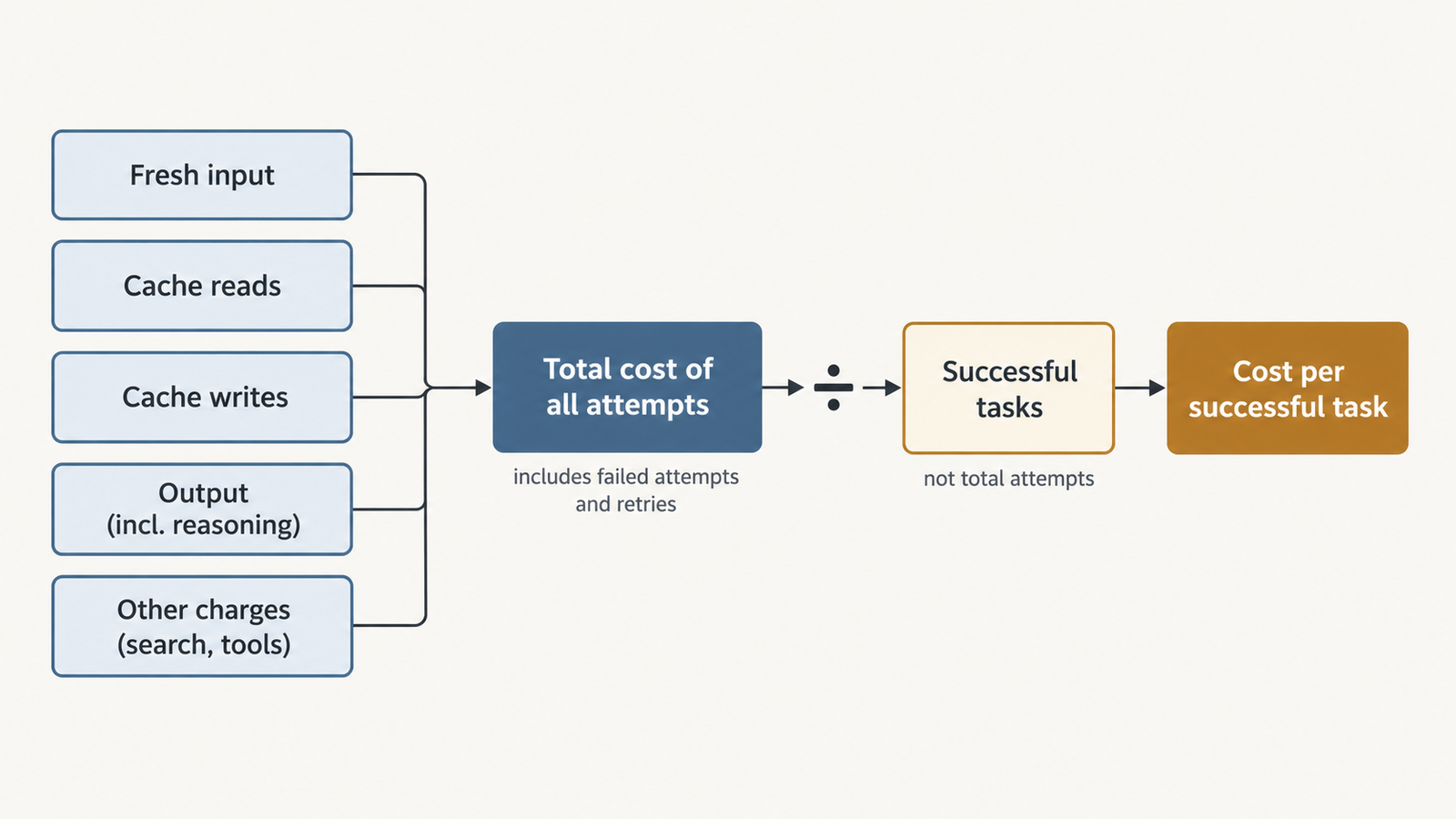
Checked against the burner22/numbat repository and its discussions, Hugging Face and PyTorch documentation, and Moonshot AI’s announcement on 2 November 2026. On 1 November, a …
Agentic AI Statistics

30 Agentic AI Statistics for 2026: Adoption, Spending and Risk

Last updated: 15 November 2026. This page is updated monthly; each figure keeps its original publication date. Agent traffic at one healthcare booking platform rose …

Agentic AI vs Generative AI: Cost, Risk and Control

agentic AI vs generative AI

Generative AI produces an output, such as text, code or an image, from a prompt and its context. Agentic AI is a system that uses a generative model to pursue a goal over several steps, calling tools and acting on the results until it finishes or is stopped.

So agentic AI vs generative AI isn’t a contest between two kinds of model. Most agents run on the same large language models (LLMs) as chat assistants. What changes is the system around the model: how many calls a task makes, what those calls may touch, what they cost together and what happens when one goes wrong. The sections below work through each difference with calculations you can rerun on your own numbers.

Key Takeaways
  • They aren’t rival model types. An agent is an application architecture that usually calls a generative model many times.
  • Repeated context dominates many agent bills. In our illustrative ten-call loop, 84% of input tokens were repeats.
  • Token price isn’t task cost. In a hypothetical comparison, a model at one-third of the token price cost about 38% more per completed task.
  • Caching helps only when it hits. Cache writes cost more than ordinary input, so a loop that keeps missing the cache pays extra.
  • Actions outlive answers. Validation, idempotency and approval gates belong outside the model.
  • Instructions aren’t permissions. Prompt injection is a risk to contain with system controls; filtering alone doesn’t remove it.
  • Known steps call for a pipeline. If you can write the workflow down in advance, fixed code with model calls at set points is usually cheaper and easier to test.

Quick Navigation


Agentic AI vs generative AI: the architectural difference

Generative AI describes a capability. Agentic AI describes how a system uses it. The two overlap, because an agent’s plans, tool choices and final answer usually come from a generative model.

Anthropic’s guide Building effective agents (December 2024) draws a useful line. Workflows are systems where “LLMs and tools are orchestrated through predefined code paths.” Agents are systems where “LLMs dynamically direct their own processes and tool usage.” The practical question is who decides the next step: your code or the model.

DimensionSingle generative callAgentic system
Unit of workOne request, one responseA task spanning many calls
Who picks the next stepThe user or calling codeThe model, within set limits
Calls per taskOneVariable, often unknown in advance
Side effectsNone unless someone acts on the outputPossible at every tool call
Main cost driverPrompt and output lengthCalls × context per call
Typical failureA wrong outputA wrong action, or a loop that never ends

The boundary isn’t absolute. Someone can paste generated SQL straight into production, and an agent can be limited to writing a report. The difference is structural: in an agent, the gap between the model’s decision and its effect is a function call, not a person.

Where the tokens go in agentic AI vs generative AI

A single request is easy to cost. An agent loop is harder, because each call re-sends material the model has already seen.

Every call carries the system instructions and tool definitions. OpenAI’s function-calling guide says function definitions “are billed as input tokens.” Anthropic’s tool-use documentation also adds a tool-use system prompt of 286 or 406 tokens on its 5.5-generation models, as listed on 18 October 2026. On top of that come the history, each earlier tool call and result, and the newest observation. Reasoning tokens, where a model produces them, are billed as output.

A worked example with illustrative assumptions

These are illustrative assumptions, not measurements of any product.

  • The system instructions take 1,500 tokens, the tool definitions 2,500 and the user task 500.
  • The one-shot request has no tools but includes a 3,000-token document, and it returns 800 tokens.
  • Each agent step outputs 300 tokens and receives a 1,500-token tool result. The final answer is 800 tokens.
  • The agent carries its full transcript forward.
  • Prices are $3 per million input tokens and $15 per million output tokens. These are round illustrative rates, not a current list price.

Call k therefore sends 4,500 tokens of prefix and task, plus 1,800 for every earlier step:

Input for call k        = 4,500 + (k − 1) × 1,800
Total input over n calls = 4,500n + 900n(n − 1)
ScenarioCallsInput tokensOutput tokensIllustrative cost
One-shot generation15,000800$0.027
Agent, five calls540,5002,000$0.152
Agent, ten calls10126,0003,500$0.431

Doubling the calls from five to ten more than tripled the input. Of the ten-call run’s 126,000 input tokens, only 20,700 were new; the other 84% were repeats.

That growth comes from the design, not from agents in general. A state-managed version might send the prefix, the task, a 500-token summary and only the latest observation. Its calls then stay at 6,500 tokens after the first, for 63,000 in total, half the transcript version. The catch is that a summary can drop a detail a later step needed.

For real-world scale, Anthropic reported that agents in its multi-agent research system (June 2025) “typically use about 4× more tokens than chat interactions,” and multi-agent systems “about 15× more.” That’s one company measuring one product.

agentic AI vs generative AI

Agentic AI vs generative AI: the cost of completing a task

Price per million tokens tells you what a call costs, not what finished work costs, because failed attempts are paid for too.

Cost per successful task = (inference + tools + infrastructure + retries)
                           ÷ successfully completed tasks

Take a hypothetical pair using the same token assumptions, plus $0.02 per attempt for tool APIs and sandbox compute. Model A costs $1 input and $5 output per million tokens, averages 18 calls and completes 60% of tasks. Model B costs $3 and $15, averages 10 calls and completes 92%.

Per 1,000 attemptsModel AModel B
Input tokens per attempt356,400126,000
Total cost$405.90$450.50
Successful tasks600920
Cost per successful task$0.677$0.490

Model A charges a third of the token price yet costs about 38% more per completed task. Longer loops absorb most of its price advantage, and the lower completion rate does the rest. The table also ignores the 400 failed tasks, and if a person picks those up, the labour can outweigh the inference bill. Our breakdown of the three numbers inside inference cost per token explains how list prices become the rate you actually pay.

What caching changes

Anthropic’s prompt-caching documentation, checked on 18 October 2026, prices five-minute cache writes at 1.25× the base input rate and reads at 0.1× for many models. The cache lasts five minutes by default, refreshed on each use, and changing tool definitions invalidates all of it. OpenAI’s caching guide describes automatic caching with a 1,024-token minimum and, for GPT-5.6 and later, the same 1.25× and 0.1× multipliers.

Apply those multipliers to the ten-call example, with each call reading the previous prefix and writing only its new tokens. The task falls from $0.431 to $0.162, about 62% less. If every step instead waits past the cache lifetime, perhaps for human approval, each call writes and none reads. The task then costs $0.525, about 22% more than with no caching. Measure your hit rate before counting on the discount.

Agentic AI vs generative AI when a step fails

A wrong answer and a wrong action differ mainly in what has already happened by the time anyone notices.

A generated output that’s wrongAn agent action that’s wrong
A summary misstates a contract termThe agent writes the wrong term into the contract record
A code suggestion has a destructive bugThe agent runs that code with production write access
A recommendation names the wrong supplierThe agent emails that supplier or calls its ordering API

The left column still needs a person to act. The right column doesn’t. The line isn’t absolute, though: people act on unchecked generated text, and a read-only agent may never change anything.

Errors also compound. Anthropic’s write-up says plainly, “Agents are stateful and errors compound.” If ten independent steps each succeed 95% of the time, all ten succeed only about 60% of the time (0.95¹⁰ ≈ 0.60). Real steps aren’t independent, so treat that as arithmetic, not a forecast.

Picture a refund agent whose database write commits but whose confirmation times out. A naive retry issues a second refund. The controls that contain this are:

  • Validation: code checks each proposed action against a schema and business rules before it runs.
  • Idempotency keys: a retried write applies only once.
  • Bounded retries: attempts are capped per step and per task.
  • Transaction boundaries: related writes commit together or not at all.
  • Approval gates: a person confirms costly or irreversible actions.
  • Compensation: each action that can’t be undone directly has a defined correcting action.
  • Audit logs: the system records what was proposed, what ran and under which identity.

Agentic AI vs generative AI: security is an execution problem

A model that follows instructions well still isn’t a security boundary. The OWASP Top 10 for LLM Applications 2025 lists Excessive Agency (LLM06) and traces it to “excessive functionality,” “excessive permissions” and “excessive autonomy.” Its fixes include “complete mediation,” meaning authorisation enforced in downstream systems rather than by the model.

Prompt injection is why. OWASP’s prompt-injection entry (LLM01) covers instructions hidden in web pages, files and other content an agent reads. It says “it is unclear if there are fool-proof methods of prevention.” The UK’s National Cyber Security Centre argued in December 2025 that prompt injection is not SQL injection. Its reasoning was that LLMs “do not enforce a security boundary between instructions and data inside a prompt.” It therefore recommended deterministic, non-LLM safeguards over filtering alone. In March 2026, NIST’s Center for AI Standards and Innovation reported a red-teaming competition with more than 250,000 attack attempts. At least one attack succeeded against each of the 13 frontier models tested.

Where the controls belong

A filter can lower the odds of an attack, but it can’t decide what an attack may do. A framework’s tool list only controls what the model can request. A “run_python” tool inside your application process inherits that process’s network access, files and credentials. Real isolation comes from the operating system, container or virtual machine, plus egress rules and per-tool credentials. Our guide to the four layers of sandbox isolation covers how each layer limits damage.

The controls that matter are:

  • Least privilege: each tool gets only the access its job needs.
  • Tool allowlists: the agent calls named, reviewed tools, with no general shell unless the task requires one.
  • Scoped credentials: each tool has its own short-lived token.
  • Egress restrictions: outbound traffic is blocked by default.
  • Sandboxing: generated code runs outside the application’s process.
  • Human approval: payments, deletions and external messages wait for a person.
  • Independent policy enforcement: a separate check decides whether each action is authorised.

No single item makes an agent secure. OWASP’s Top 10 for Agentic Applications (December 2025) lists Agent Goal Hijack, Tool Misuse, Identity & Privilege Abuse and Cascading Failures as separate risks. Each needs its own control.

agentic AI vs generative AI

Agentic AI vs generative AI under rate limits

Four measures get confused. Requests per minute (RPM) counts API calls. Tokens per minute (TPM) counts text processed. In-flight concurrency is how many requests are open at once, and end-to-end latency is how long the user waits.

Providers measure these differently. On 18 October 2026:

  • OpenAI sets RPM, TPM and daily limits per organisation and project. Its guide warns that “unsuccessful requests contribute to your per-minute limit.”
  • Anthropic sets RPM and separate input and output TPM per model class. Its documentation says cache reads don’t count toward input limits for most models.
  • Google’s Gemini API applies RPM, TPM and daily limits per project, not per key, and says they “are not guaranteed.”
An illustrative fan-out

Suppose 100 users start a task in the same minute, using the five-call agent above. Each of its four tool steps runs three tools in parallel. Each model call takes 6 seconds and each tool step 2 seconds.

In that minuteSingle callFive-call agent
Model requests100500
Input tokens500,0004,050,000
Downstream tool calls01,200
Time per taskabout 6 secondsabout 38 seconds

The agent sends five times the requests and about eight times the input tokens, and it also loads your own systems, such as a search API or CRM. With caching on a provider that excludes cache reads, the input counted against limits drops to about 1.17 million, but the request count doesn’t change.

Retries can make this worse, because immediate retries after 429 errors add requests to a minute that’s already full. Honour any retry-after header, and otherwise use exponential backoff with random jitter, which Marc Brooker’s AWS analysis showed cuts wasted work sharply. Agents also need bounded concurrency per model and tool, a queue that holds new tasks instead of failing them, cancellation of abandoned branches, and hard caps on steps, time and tokens. Our reference on AI API rate limits in 2026 compares each provider’s published ceilings.

When a pipeline beats an agent

Anthropic’s advice is to find “the simplest solution possible,” because agentic systems “trade latency and cost for better task performance.” That trade only pays when you need the performance.

A deterministic pipeline is the better choice when you can list the steps in advance, check each output in code, run at high volume, or meet a tight latency budget. Pipelines still use generative models: one call classifies a ticket, another extracts fields, and a third drafts the reply, with code fixing the order.

Agents earn their cost when the next step depends on what the last one found, as in debugging or open-ended research. Even then, a bounded agent often works best. It has narrow tools, a step limit and deterministic checks before any write, and it sits inside a larger pipeline.

A practical decision table

ScenarioLikely architectureWhy it fitsMain concern
Single-turn drafting and summarisationOne model callThe output is the product, and a person reviews itAccuracy
Structured extraction and classificationPipeline with schema validationFixed steps; output checkable in codeSilent field errors at volume
Research across several sourcesBounded agent with read-only toolsThe next search depends on the last resultToken growth; injected content
Database updates and external transactionsPipeline, or an agent that only proposes, with approval and idempotent writesSide effects must be validated and reversibleDuplicate or unauthorised writes
Long-running multi-step workflowsWorkflow engine with agent steps insideState and retries belong in infrastructureCache expiry, lost state, runaway loops
High-volume, latency-sensitive requestsSingle call or short fixed chainPredictable latency and limitsFan-out and retries under load

Conclusion

The difference between agentic AI and generative AI shows up in operations more than output. An agent multiplies calls, compounds errors, holds permissions and loads rate limits in ways a single generation doesn’t.

So use one model call when one output answers the request, and a pipeline when you can write down the steps. Use an agent only when the next step depends on what the last one found. Then give it a step limit, a token budget, scoped credentials and a checker that isn’t the model.

FAQ

What is the difference between agentic AI and generative AI?

Generative AI produces content from a prompt. Agentic AI is a system that pursues a goal over several steps, choosing actions, calling tools and using the results. Agents usually rely on a generative model to decide.

Can generative AI become part of an agentic system?

Yes, and it usually does. The model plans, picks tools and writes the answer, while the application runs the loop, executes tools and enforces limits.

Is agentic AI more expensive than generative AI?

Usually, per task, because one task triggers many calls that re-send context. Caching, state management and completion rate can matter more than token price.

Is agentic AI more dangerous than generative AI?

Its risks are different. An agent can act without a person in between, so mistakes and injected instructions can have direct effects. The risk scales with the permissions the system grants.

When should a company use a deterministic workflow instead of an AI agent?

Use one when the steps are known in advance, outputs can be checked in code, or volume and latency demands are high. Use an agent when the path truly depends on intermediate results.

How do you measure the cost of an agentic AI task?

Divide total inference, tool, infrastructure and retry costs by the number of successfully completed tasks. Track calls per task, tokens per call, cache hit rate and completion rate separately.

How can developers limit an AI agent’s permissions and actions?

Give each tool scoped, short-lived credentials, and run generated code in a sandbox with outbound traffic blocked by default. Require human approval for consequential actions, enforce authorisation outside the model, and cap steps, time and tokens.


Keep reading

AGI vs superintelligence

AGI vs Superintelligence: A New Name Isn’t a New Intelligence

Facts checked against official documents and reporting on 18 November 2026. On 29 September, the White House told federal agencies to stop writing “artificial intelligence” …
AI Coding Agent

AI Coding Agents Are Getting Expensive. Who’s Paying for the Tokens?

Pricing checked on official vendor pages on 17 November 2026. All USD. Cost scenarios are illustrative and labelled as such. On 28 October, TechCrunch published …
Model Weights

Verify Model Weights: 7 Checks Before You Download
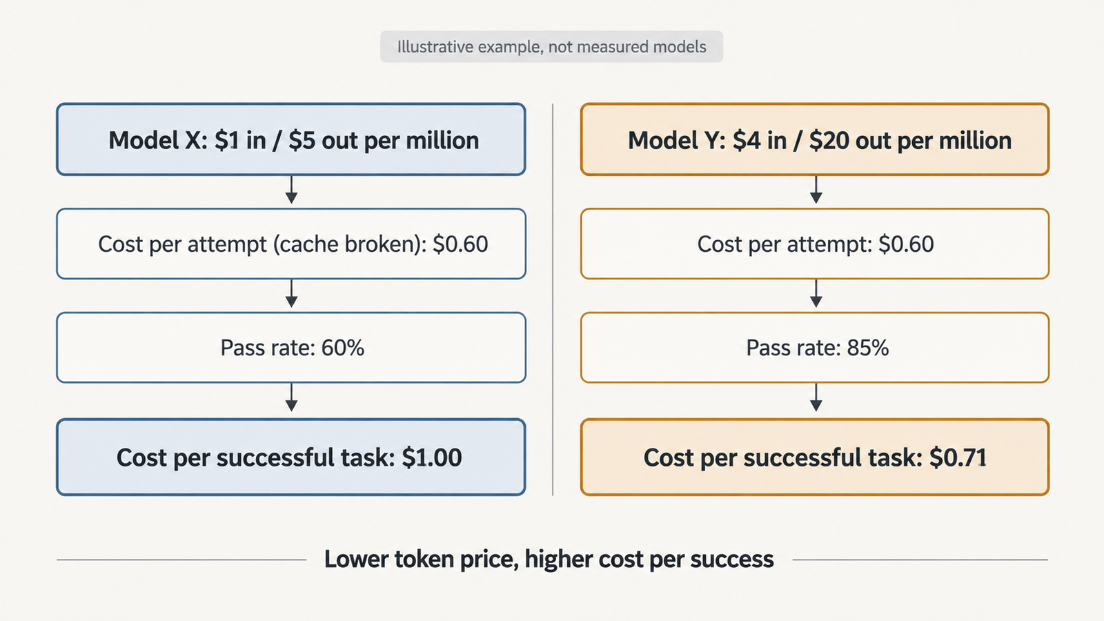
Checked against the burner22/numbat repository and its discussions, Hugging Face and PyTorch documentation, and Moonshot AI’s announcement on 2 November 2026. On 1 November, a …
Agentic AI Statistics

30 Agentic AI Statistics for 2026: Adoption, Spending and Risk

Last updated: 15 November 2026. This page is updated monthly; each figure keeps its original publication date. Agent traffic at one healthcare booking platform rose …

AMD’s Hybrid AI Math: What the 40–60% Savings Model Assumes

Hybrid AI TCO

AMD says a fleet of 500 AI PCs running half their AI work locally can cost 40 to 60% less over three years than doing all of it through cloud APIs. The company built a calculator to show the arithmetic, which is more than most vendors do.

So the number is checkable. The question is what had to be true to produce it.

Run AMD’s Tokenomics Calculator at its defaults and three assumptions carry most of the weight: a daily token volume that only heavy agentic users reach, prompt caching switched off on the cloud side, and a local model whose quality the tool explicitly declines to compare. Change any one and the percentage moves substantially.

None of that makes the model dishonest. AMD discloses its assumptions more thoroughly than the headline suggests, including a frank exclusions list. But a modeled result under stated assumptions is not a property of hybrid AI, and the useful exercise for a buyer is working out which of those assumptions describe their own workload.

Key takeaways
  • The 40–60% figure is a modeled outcome for one scenario: 500 users at the Medium workload tier, 50% hybrid mix, three-year horizon, July 2026 cloud prices. It is not a general property of hybrid deployment.
  • The Medium tier assumes 5.74 million input and 574,000 output tokens per user per day — roughly 200 input tokens per second sustained across an eight-hour day. That is continuous agent activity, not assisted office work.
  • Prompt caching is supported in the calculator but off by default. Enabling it on a repetitive agentic workload can cut cloud input costs dramatically, which is the single biggest threat to the headline result.
  • At a 50% hybrid mix the calculator buys hardware for every user and runs half the tokens locally. The capital cost is full; the local utilisation is not.
  • AMD states plainly that the calculator does not consider performance needs and excludes model-quality differences, software licensing, IT management, migration, taxes, financing and egress.
  • Local throughput is measured on a quantised 35B open model. Comparing its cost against Claude Opus or GPT 5.5 pricing compares two different things.
  • The defensible conclusion: hybrid AI TCO can produce real savings for high-volume, repetitive, quality-tolerant workloads. Whether it does for you is a measurement question, not a percentage you can inherit.

Quick Navigation


What AMD’s Calculator Actually Models

Hybrid AI TCO is the total cost of running AI workloads across a mix of local hardware and cloud APIs, counting hardware, electricity and token charges over a defined period. AMD’s Tokenomics Calculator models three paths — cloud only, local on AMD devices, and a hybrid split — and reports three-year totals, monthly run rates and break-even months.

The inputs it takes:

InputOptions
Team size25, 250, 1,000 or custom
Analysis period1, 3, 4 or 5 years
Workload tierLight, Medium, Heavy or custom, as tokens per user per day
Cloud model mixGemini Pro $2/$12, Claude Sonnet $3/$15, Claude Opus $5/$25, GPT 5.5 $5/$30, or custom, per million tokens
Hybrid mix0% to 100% local
HardwareRyzen AI 9 HX 470, Ryzen AI Max+ 395, Radeon AI PRO R9700, with editable price, throughput, power and hours per day
EnergyElectricity rate and powered days per month
Cloud modifiersPrompt caching, batch discount, regional multiplier, long-context premium, monthly API surcharge

That is a more complete model than the headline implies, and the advanced panel exposes nearly every assumption for editing. Credit where it is due: the caching, batch and long-context controls exist, and most vendor calculators do not have them.

Three mechanics in the fine print matter more than anything on the main panel.

  1. Cloud cost is API tokens only. AMD states there is no seat, subscription or flat monthly price in the cloud figure. For an organisation actually paying per-seat for a coding assistant, this models a different cost structure than the one on their invoice — sometimes higher, sometimes lower.
  2. Hybrid buys hardware for everyone. At 50% mix, all users get a device and half the token volume runs on it. The hardware line is identical to a full local deployment.
  3. Hardware life equals the analysis period. Choose three years and the full device cost lands inside three years, adjusted by an end-of-life value percentage. There is no refresh cycle and no residual beyond that field.

AMD also prices local throughput from a specific measurement: Qwen 3.6 35B A3B at Q4_K_M quantisation, 262,000-token context prefilled to 128,000, sustained throughput under Vulkan llama.cpp. That is a real benchmark configuration, disclosed, and it is the quiet centre of the whole comparison — because it is the model whose cost is being compared against Claude Opus pricing.

The Token Assumption Does Most of the Work

5.74 million input tokens per user per day sounds abstract. Convert it and it stops being abstract.

Our calculations from AMD’s stated tier, using an eight-hour working day and 260 working days.

UnitInput tokensOutput tokens
Per day5,740,000574,000
Per hour (8h day)717,50071,750
Per second sustained~199~20
Per year~1.49bn~149m
Per 500-user fleet, per year~746bn~75bn

Two hundred input tokens per second, sustained, for every second of every working hour. That is not a person typing prompts. That is an agent running continuously, reading a repository, re-sending context and looping through tool calls.

For scale, 5.74 million tokens is in the region of four million words of input per person per day. No human reads or writes that. Only a machine loop produces it.

Three workload profiles, to show the spread. These are illustrative sketches, not measured data.

ProfileWhat it looks likeRough daily input tokens
Light office AIDrafting, summarising, occasional questionsTens of thousands to low hundreds of thousands
Knowledge worker with AI assistanceRegular use, document context, some retrievalHundreds of thousands to low millions
Continuous agentic codingCoding agent with large repo context, long sessionsMillions to tens of millions

AMD’s own Light tier sits at 574K input, a tenth of Medium. The gap between those two tiers is roughly the gap between a typical office deployment and a developer running a coding agent all day.

Why this dominates the result: cloud cost scales linearly with tokens while hardware cost is fixed. At the Medium tier on Claude Sonnet pricing, one user’s input tokens alone come to roughly $4,470 a year, with output adding about $2,240 — call it $6,700 per user per year, or $20,000 over three years. That is our arithmetic at AMD’s stated tier and prices. Against an AI PC costing one to three thousand dollars, the comparison is not close.

Drop to the Light tier and the same arithmetic yields roughly $670 per user per year. Now a $2,000 device takes about three years to pay for itself before counting electricity, management or anything AMD excludes, and the 40–60% headline does not survive.

The lesson is not that AMD picked an unfair number. It is that tier selection, more than hybrid mix, determines the answer. A buyer starting from the default tier rather than their own metered token volume is reading somebody else’s workload.

Where Prompt Caching Changes the Cloud Side

Here is the tension at the centre of the model. The workload that justifies the Medium tier — a continuous agent re-sending large context — is precisely the workload that prompt caching was designed for.

An agent turn is mostly repetition: the same system instructions, the same tool schemas, the same repository or document context, plus a small amount of genuinely new input. Providers price reused prefixes far below fresh input, and the discount is steep. On current frontier pricing, cached reads land near $0.20 per million tokens against input rates of $2 to $5. We worked through what that does to real bills in our analysis of the cache line that decides agentic costs.

AMD’s calculator supports this. The advanced panel has cache write share, cache read share, a write multiplier (1.25x for a five-minute window, 2x for an hour) and a read multiplier. The controls are there and they are correctly specified.

They are also off by default.

What that means in practice: the following is our illustrative arithmetic, not a calculator output. Take the Medium tier’s 5.74M daily input tokens on Claude Sonnet at $3 per million.

Cache-hit rateEffective input cost per user per dayAnnual input cost per user
0% (calculator default)$17.22~$4,477
50%$9.47~$2,462
80%$4.82~$1,253
90%$3.27~$850

At a 90% hit rate, the cloud input bill falls by roughly 80%. Since input dominates this workload’s token volume, that reshapes the entire comparison — and it reshapes it in the direction that hurts the local case.

The honest counterweight: high cache-hit rates are not automatic. They depend on prefix stability, on how the agent structures its context, on cache window duration against request frequency, and on provider implementation. An agent that rebuilds its context every turn gets little benefit and pays cache-write premiums for the privilege. Assuming 90% is as wrong as assuming zero.

So the correct criticism of AMD’s default is narrow and fair: for the specific workload profile that makes the Medium tier plausible, zero caching is the least likely assumption, and it is the one the tool ships with. Any buyer running this calculator should turn caching on and enter their own measured hit rate before reading the savings number.

The Utilisation Problem on the Local Side

The cloud side of this comparison is perfectly elastic: you pay for tokens consumed and nothing else. The local side is the opposite. You buy a device, and whether it earns its price depends entirely on how much work passes through it.

The calculator handles this more carefully than most. It has an “hrs/day running AI” field per device, it sizes capacity from throughput times that window, and it warns when fleet capacity falls short of token demand. Those are the right mechanics.

What the default scenario still implies is worth making explicit. At a 50% hybrid mix, every user gets a device and half the token volume runs on it. The device’s economic output is therefore half what the same hardware could produce — while its cost is unchanged. In utilisation terms, a 50% hybrid mix is a 50%-utilised fleet, at best.

Hybrid AI TCO

The gap between purchased and productive capacity has several sources, and they compound:

  • AI-active hours are not working hours. A device powered for eight hours may run inference for two.
  • One device per user caps sharing. The calculator states a hard ceiling of one device per user. A heavy user cannot borrow a colleague’s idle capacity.
  • Nights and weekends are free capacity nobody uses. Unless batch or background agent work is scheduled into them, two thirds of each day is idle.
  • Provisioning follows the peak. Hardware sized for the busiest user is over-provisioned for everyone else.
  • Adoption is uneven. Fleet-wide deployment assumes fleet-wide usage. Actual AI adoption inside organisations is famously lumpy.

This is the same economics we set out in our analysis of accelerator utilisation: once capacity is bought rather than rented, idle time stops being an efficiency question and becomes a cost-per-unit question. Every hour the device does not run inference raises the effective cost of the hours it does.

The flip side deserves equal weight, because it is the strongest argument for the local case. A device that runs background agents overnight, processes batch jobs on weekends, or serves a developer who genuinely saturates it can reach utilisation a cloud buyer pays dearly for. Local capacity has no marginal token cost. If you can fill it, you should.

The practical test is simple: measure AI-active hours per user, not headcount. A fleet where ten per cent of staff generate ninety per cent of token volume should not be deployed uniformly, and uniform deployment is exactly what the calculator’s hybrid model assumes.

The Missing Variable: Model Quality

AMD says this plainly, twice, and it deserves to be quoted rather than discovered: the calculator does not consider your performance needs, and model inference quality differences are excluded.

That exclusion is doing a lot of work, because of what is on each side of the comparison. The cloud column is priced from Claude Opus, GPT 5.5, Claude Sonnet or Gemini Pro. The local column is throughput-measured on Qwen 3.6 35B A3B at four-bit quantisation. Both are real. They are not the same capability, and the calculator compares their costs without comparing their outputs.

The economic principle is the one that matters here, and it generalises well beyond AMD:

Cost per token is not cost per completed task.

A cheaper model that needs more attempts can cost more in total. Work the chain through:

  • A task that takes two attempts instead of one doubles the token volume for that task
  • A task that needs human review consumes the most expensive resource in the building
  • A wrong output that reaches a downstream system costs far more than either
  • A longer reasoning path to the same answer burns more tokens on cheaper hardware

The arithmetic that follows is unforgiving. If a local model completes 70% of tasks that a frontier model completes at 95%, the effective cost per completed task rises by roughly a third before counting retries — and that is before anyone prices the human time spent on the failures.

None of this says local models are inadequate. Open models at 30B-class sizes have become genuinely capable, and for classification, extraction, summarisation, routing and structured transformation they are often indistinguishable from frontier models at a fraction of the cost. That is a real and growing category of work.

The point is narrower: a TCO model that excludes quality is answering “what does this cost?” rather than “what does this deliver per pound spent?” For the tasks where the two models are equivalent, AMD’s comparison is fair. For the tasks where they are not, the cost column is measuring the wrong thing — and the calculator cannot tell you which tasks are which. Only your own evaluation can.

Why 50/50 Is a Modeling Choice, Not a Strategy

The hybrid mix slider defaults to 50%. It is a reasonable midpoint for a demonstration and a poor description of how workloads actually divide.

Real routing is decided by task characteristics, not by percentages:

Route locallyRoute to cloud
Classification, extraction, taggingComplex multi-step reasoning
Summarisation of routine documentsNovel problem-solving
Privacy-sensitive or regulated dataTasks needing the newest model capabilities
High-volume repetitive transformationBurst workloads above local capacity
Offline or air-gapped workAnything where a wrong answer is expensive
Draft generation before human editingFinal output that ships unreviewed

Run that split against a real workload and the local share lands wherever it lands — 15%, 40%, 80%. The number is an output of the routing policy, not an input to it. An organisation doing mostly structured data work might route 80% locally. One doing mostly open-ended analysis might manage 20%.

This also explains why the calculator’s “max potential savings at 100% hybrid” figure should be read carefully. Full local means no access to frontier capability at all, which is a product decision rather than a cost optimisation.

What AMD’s Model Gets Right

Credit where it is earned, because the tool is better than the headline it generated.

  • It discloses its assumptions. Token tiers, model prices with a date, electricity rate, throughput test configuration, device specs — all visible and editable.
  • It publishes an exclusions list. Model quality, licensing, IT management, migration, taxes, financing, egress, volume discounts. Most vendor calculators omit this entirely.
  • It includes the modifiers that matter. Caching, batch discounts, long-context premiums and regional multipliers are all present, even if off by default.
  • It flags capacity shortfalls. If the fleet cannot serve the token demand, it says so and routes the overflow to cloud.
  • It states its own limitation on performance. “This calculator does not consider your performance needs” is an unusually honest sentence to put in a sales tool.
  • The underlying economics are sound. For sufficiently high, sufficiently repetitive token volumes, local inference genuinely is cheaper. That is not marketing; it is arithmetic.

What It Leaves Out That Could Matter

The exclusions are disclosed, but not all of them are equally consequential. Ranked by how much they could move a real result:

ExclusionWhy it mattersDirection
Model qualityChanges cost per completed task, not cost per tokenUsually favours cloud
Caching, when left offOverstates cloud input costs on repetitive workloadsFavours local as shipped
IT management and supportManaging local inference across a fleet is real workFavours cloud
Software licensingLocal serving stacks, management tooling, model licencesFavours cloud
Migration and deploymentOne-off but substantial for a 500-device rolloutFavours cloud
Hardware refreshLife is set to the analysis period; a 5-year window assumes 5-year devicesFavours local as shipped
Volume discountsEnterprise cloud agreements rarely pay list priceFavours cloud
Seat and subscription pricingMany organisations pay per seat, not per tokenDepends
Utilisation below 100%Capacity bought is not capacity usedFavours cloud

Notice the pattern. Most of the exclusions push in the same direction, and it is not the direction that makes local hardware look better.

A Better Hybrid AI TCO Calculation

Ten steps. The first four are measurement, and skipping them is how buyers end up with somebody else’s answer.

  1. Meter your actual token consumption. Pull it from provider dashboards or your gateway logs, not from headcount multiplied by an assumption.
  2. Separate input from output. They price differently and they scale differently. Input dominates agentic work; output dominates reasoning work.
  3. Measure your cache-hit rate. Most providers report cached-token usage. This single number may move your cloud bill more than any hardware decision.
  4. Measure AI-active hours per user, not working hours, and look at the distribution rather than the average.
  5. Classify tasks by quality requirement. Which actually need a frontier model? Test, do not assume.
  6. Calculate realistic local utilisation. Include nights, weekends and the users who barely touch AI.
  7. Add the omitted costs. Management, support, licensing, migration, refresh.
  8. Compute cost per completed task for both paths, including retries and human review.
  9. Test several routing mixes — 0%, 25%, 50%, 75%, 100% — rather than accepting the default.
  10. Run sensitivity on your two or three largest variables and see how wide the range gets.

Sensitivity: Which Assumptions Move the Answer

Directional, based on the model’s structure rather than on outputs we cannot reproduce exactly.

If this changesLocal and hybrid TCOWhy
Token volume risesImproves sharplyCloud scales linearly, hardware does not
Token volume fallsDeteriorates sharplyFixed hardware cost spread over less work
Cache-hit rate risesDeterioratesCloud input cost falls, sometimes by 80%+
Local utilisation risesImprovesSame capital, more output
Cloud API prices fallDeterioratesThe savings baseline shrinks
Electricity price risesDeteriorates mildlyPower is a small share at these volumes
Hardware price fallsImprovesLower capital to amortise
Quality requirements riseDeterioratesMore work must route to cloud regardless of cost
Refresh cycle shortensDeterioratesCapital amortised over fewer years
Hybrid mix rises toward 100%Improves on cost, narrows on capabilityFewer tokens billed, less frontier access

The two largest levers are token volume and cache-hit rate, and they pull in opposite directions on the same workload. That is the central tension in AMD’s model: the workloads with enough tokens to justify local hardware are the workloads most likely to benefit from caching.

FAQ

What is hybrid AI TCO?

The total cost of running AI workloads across both local hardware and cloud APIs over a defined period, counting hardware purchase, electricity and token charges. It differs from cloud-only TCO because part of the cost becomes fixed capital rather than metered usage.

Can hybrid AI really reduce AI costs by 40–60%?

AMD’s calculator produces that result for a specific scenario: 500 users at 5.74 million input and 574,000 output tokens per user per day, a 50% local mix, a three-year horizon and July 2026 cloud prices with prompt caching off. Under those assumptions the arithmetic holds. Whether it holds for a given organisation depends on whether its workload resembles that profile.

Is local AI cheaper than cloud AI?

For high-volume, repetitive, quality-tolerant workloads on well-utilised hardware, frequently yes. For light or intermittent usage, usually no, because fixed hardware cost is spread across too little work. The crossover point is set by token volume, utilisation and the cache-hit rate on the cloud side.

How does prompt caching affect hybrid AI TCO?

Significantly, and against the local case. Cached input tokens are priced far below fresh ones, so a repetitive agentic workload with a high hit rate can cut its cloud input bill by most of its value. AMD’s calculator supports caching but ships with it disabled, which prices every input token at full rate.

How much does AI PC utilisation affect TCO?

Proportionally. A device used half as much has roughly double the effective cost per unit of work, since the purchase price does not change. At a 50% hybrid mix the calculator buys hardware for every user and runs half their tokens locally, which is a 50%-utilised fleet by construction.

What costs are missing from AMD’s AI cost calculator?

AMD lists them: model inference quality differences, software licensing, IT management, migration effort, taxes, financing fees, network and egress costs unless entered manually, and provider-specific volume discounts. Most of these, if included, would favour the cloud side.

Is a 50/50 local and cloud split optimal?

It is a default, not an optimum. The right mix follows from task routing — which work genuinely needs frontier capability and which does not — and lands anywhere from 15% to 80% local depending on the workload.

How should businesses calculate AI TCO?

Start by metering actual token consumption split into input and output, measure the cache-hit rate and AI-active hours per user, classify which tasks need frontier models, then compute cost per completed task for several routing mixes rather than cost per token for one.

Does AMD’s calculator compare equivalent models?

No, and it says so. Local throughput is measured on Qwen 3.6 35B A3B at four-bit quantisation, while cloud costs are priced from Claude, GPT and Gemini models. AMD states explicitly that the tool does not consider performance needs.


Keep reading

AGI vs superintelligence

AGI vs Superintelligence: A New Name Isn’t a New Intelligence

Facts checked against official documents and reporting on 18 November 2026. On 29 September, the White House told federal agencies to stop writing “artificial intelligence” …
AI Coding Agent

AI Coding Agents Are Getting Expensive. Who’s Paying for the Tokens?

Pricing checked on official vendor pages on 17 November 2026. All USD. Cost scenarios are illustrative and labelled as such. On 28 October, TechCrunch published …
Model Weights

Verify Model Weights: 7 Checks Before You Download

Checked against the burner22/numbat repository and its discussions, Hugging Face and PyTorch documentation, and Moonshot AI’s announcement on 2 November 2026. On 1 November, a …
Agentic AI Statistics

30 Agentic AI Statistics for 2026: Adoption, Spending and Risk

Last updated: 15 November 2026. This page is updated monthly; each figure keeps its original publication date. Agent traffic at one healthcare booking platform rose …