Gemini 4 Carbon Is Here. But Can You Actually Use It?

Gemini 4 Carbon

Published 30 October 2026. Access, pricing and benchmark details verified on 30 October. Sections 2, 6 and 8 will be updated as Google expands access.

Gemini 4 Carbon now leads the Artificial Analysis Intelligence Index, and Google reports the strongest cybersecurity scores it has published for any model. Almost nobody can use it. Since its announcement on 28 October, Carbon has been limited to “a subset of cyber defenders”, with more trusted partners to follow through Google DeepMind’s Fairwind Program. Google hasn’t given a date for developers, businesses or consumers.

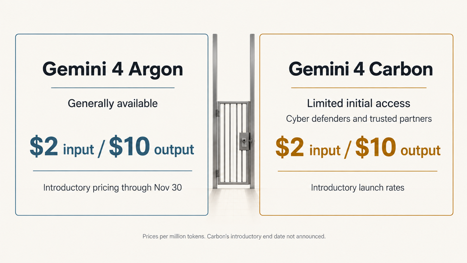
So the short answer is no: unless your organisation has been invited, you can’t call Gemini 4 Carbon today. Gemini 4 Argon, its predecessor, has been generally available since 13 October and is the model you can build on now. The more useful question is what an Argon team should do while it waits. Carbon’s launch price and Argon’s 1 December price rise make that more pressing than it looks.

Key Takeaways
  • Carbon isn’t publicly available. Access is limited to selected cyber defenders, then Fairwind partners. It has no public model ID and no listing on the Gemini API pricing page as of 30 October.
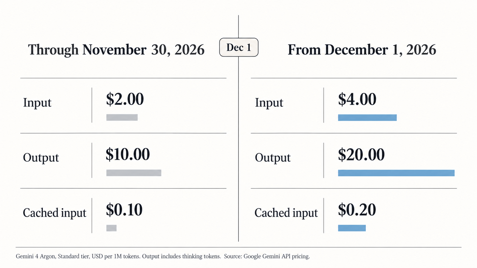
  • Argon is the model you can use. It’s a stable Gemini API model at $2 input and $10 output per million tokens until 30 November, then $4 and $20.
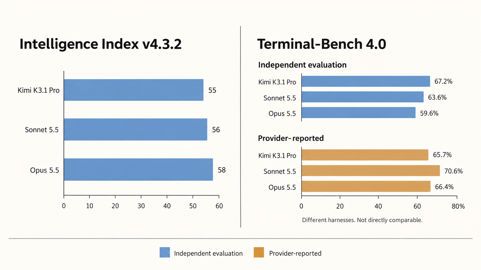
  • Carbon’s lead is real on Artificial Analysis. It scores 59 at High effort, against 50 for Argon and 52 for Claude Opus 5.5 at the same setting.
  • The cyber scores are Google’s own, measured without guardrails. SEC-bench Pro tests reproducing known bugs, not discovering new ones.
  • Don’t rebuild around a model you can’t call. Keep Argon in production, put model choice behind a configuration switch, and keep an evaluation set ready for Carbon.

Quick Navigation


What Gemini 4 Carbon’s announcement changes

Google DeepMind’s Koray Kavukcuoglu introduced Carbon as “our strongest model with state-of-the-art cybersecurity and long horizon capabilities”. The pitch has two parts. One is security work: finding, exploiting and patching vulnerabilities. The other is long-running engineering: Google says Carbon has worked internally for days on multi-step tasks, such as root-causing and fixing bugs across large codebases.

The timing is awkward for anyone who just adopted Argon. Argon was announced on 30 September through the same cyber-defender route and reached the Gemini app and the paid API on 13 October. Carbon arrived 15 days later and is described as Argon’s successor. Teams that spent the past fortnight integrating Argon are now reading about a better model in the same family.

What hasn’t changed is what you can deploy. Every number in Carbon’s announcement describes a model most readers can’t call yet.

Can you use Gemini 4 Carbon right now?

No, not unless Google has invited your organisation. Google says Carbon is available from the week of 28 October to “a subset of cyber defenders”, with access to be “phased to additional trusted partners” through the Fairwind Program. Broader availability for developers, businesses and consumers will come “as soon as possible”. No date has been given.

The two groups aren’t the same. The first wave is a hand-picked subset of defenders. Fairwind is a standing application programme. Its public page says it prioritises governments, national cyber authorities, critical-infrastructure operators, core technology platforms and academic defensive-research labs. It works with more than 650 partners and vets applicants, including background checks. Partners must use phishing-resistant multi-factor authentication, limit access to internal security teams and must not resell or share access. As of 30 October, that page still describes Fairwind access in terms of Argon, so Carbon-specific terms haven’t been published.

For everyone else, three practical facts matter:

  • No model ID. Carbon has no published identifier, and it isn’t on the Gemini API pricing page. Any code written today would be guesswork.
  • No public API. Artificial Analysis notes that its Carbon price and speed figures are estimates for that reason.
  • Argon is the deployable option. Its model page lists gemini-4-argon as a stable model with Batch, Flex and Priority inference and a shared 1M-token context window.

Google also says Carbon went through the US government’s voluntary pre-release testing process. That helps explain the pace. A staged rollout gives Google time to watch how a strong security model is used before opening the API.

Gemini 4 Carbon vs Argon: the comparison that matters
Same price, different access
Gemini 4 ArgonGemini 4 Carbon
Announced30 September 202628 October 2026
AvailabilityGenerally available since 13 October (Gemini app, paid API)Selected cyber defenders, then Fairwind partners; no general date
Model IDgemini-4-argon (stable)Not published
Intended useGeneral frontier model, strong on securityStrongest Gemini model; long-horizon engineering and cyber defence
Artificial Analysis Index v5.0 (High)5059 (ranked first)
Cost per Index task (AA estimate)$7.68$7.76
Cyber benchmarksGoogle cites relative gains only, e.g. more than 2× on an internal secure-code testSEC-bench Pro 88.2%, ExploitGym 54.8%, CWE-bench 71.0% (Google-reported)
Gray Swan indirect prompt injection0.7% attack success (Google-reported)0.0% (Google-reported)
Price, per million tokens$2 / $10 until 30 Nov; $4 / $20 from 1 Dec$2 / $10 introductory; $4 / $20 afterwards; end date not stated
Developer readinessProduction-readyNot yet callable

The independent row is the one to read first. Artificial Analysis scores Carbon 59 and Argon 50, both at High effort, on its nine-evaluation v5.0 index. The headline “Carbon beats Opus 5.5” story needs a qualifier: Claude Opus 5.5 scores 58 at maximum effort but 52 at High. At matched settings, Carbon’s lead is wider than the leaderboard’s top two rows suggest.

The cost row is the surprise. Priced at the same $4/$20 standard rates, Carbon cost $7.76 per index task against Argon’s $7.68. It used slightly more output tokens per task, 123,000 against 116,000, and scored nine points higher. If that holds on real workloads, Carbon would deliver more capability for nearly the same spend per task. That’s a reason to test it when you can, not a reason to stop shipping on Argon now.

We haven’t put Argon’s cyber benchmark scores in the table because Google hasn’t published comparable ones. Its Argon post shows results only in chart images, and apart from Gray Swan, Carbon’s post compares against Argon only in relative terms.

What Gemini 4 Carbon’s cybersecurity scores measure

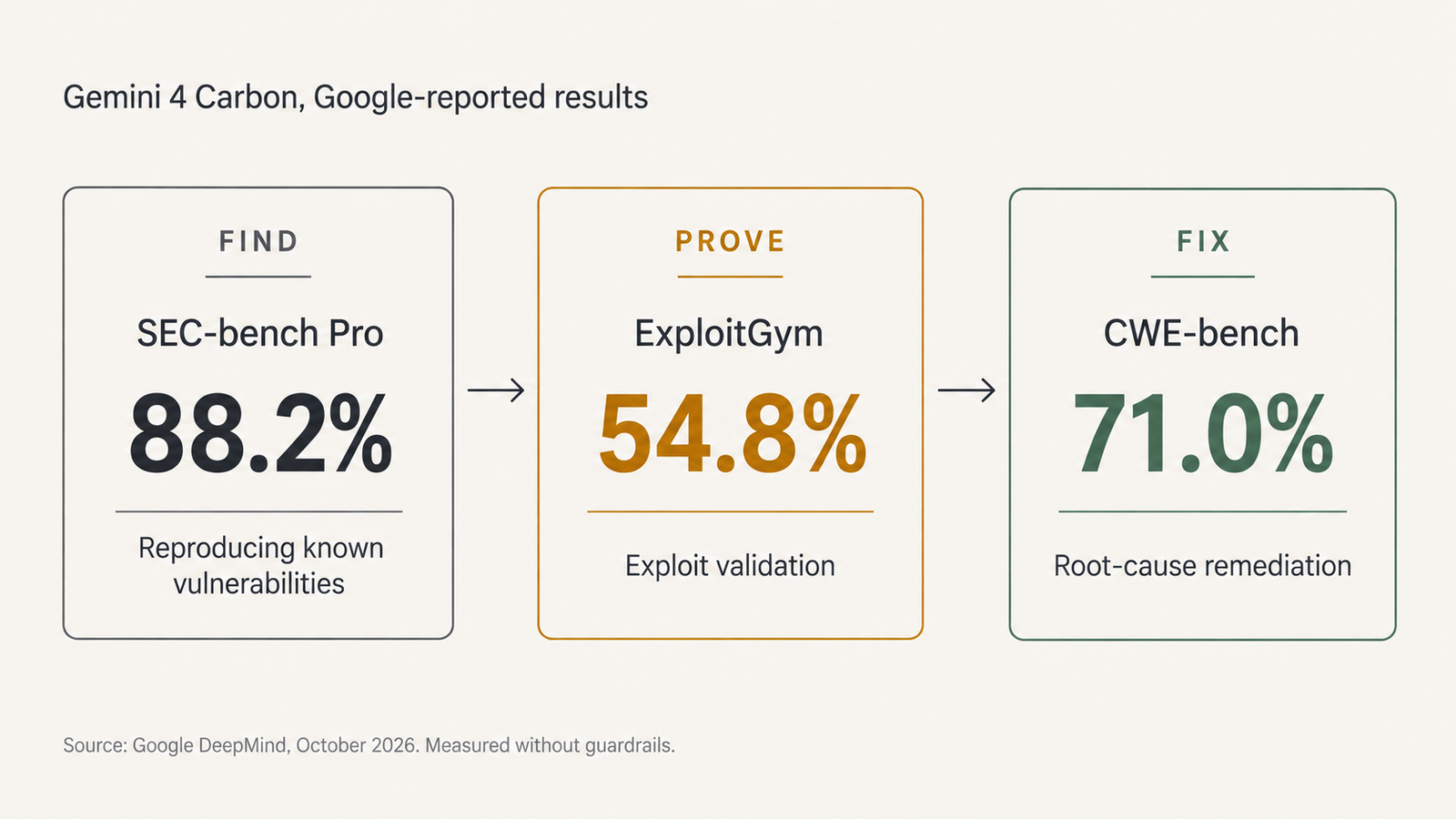
Google arranges its security results along the defender’s workflow: find a flaw, prove it matters, fix it. All three numbers are Google’s own, and its announcement says the external benchmarks were run “without guardrails”. That’s the right way to measure capability and the wrong way to estimate what a guarded production deployment will do.
Find, Prove, Fix
Find: SEC-bench Pro, 88.2%

The name suggests hunting for unknown bugs, but SEC-bench Pro measures something narrower. Its 344 tasks give a model a disclosed vulnerability in V8, SpiderMonkey or the Linux kernel, with the report, and ask it to produce a proof-of-concept input that triggers the bug. In the paper’s own runs, the best agent, Codex with GPT-5.5, solved 58%. Google reports 88.2% for Carbon. That’s a large jump in turning a bug report into a reproducer, which is real, tedious defender work. It isn’t evidence that Carbon finds zero-days at that rate.

Prove: ExploitGym, 54.8%

ExploitGym, from Berkeley’s RDI and collaborators including Google, OpenAI and Anthropic, asks an agent to turn a known vulnerability into a working exploit that captures a flag. Its 898 tasks span userspace C/C++ programs, V8 and the Linux kernel. In the May paper, the best agent captured 157 flags, about 17%, with protections such as ASLR switched off. Google’s 54.8% for Carbon is far higher. Google hasn’t said which task subset, time limit or mitigation settings it used, and those choices can move the score a lot.

Exploitation sounds like the attacker’s job, and it is also the defender’s. A proven exploit separates the bug that has to be patched tonight from the one that can wait for a release cycle.

Fix: CWE-bench, 71.0%

Collinear’s CWE-bench grades agents on repairing weaknesses across a codebase, not just the instance they were shown. Its launch example gave no credit to agents that patched a known token-revocation path but missed a newly introduced one. At launch in September, no agent repaired a majority of tasks, and the leader scored 47%. Google reports 71.0% for Carbon. This is the most directly useful of the three scores for most security teams.

Prompt injection: Gemini 4 Carbon’s Gray Swan result

On Gray Swan’s indirect prompt-injection benchmark, Google reports a 0.0% attack success rate for Carbon, down from Argon’s 0.7%. That measures how often hidden instructions in content the model reads succeed against a specific attack set. It’s encouraging for agents that browse or read email. A zero on a benchmark still isn’t a guarantee, as our piece on hidden flaws in a passing red-team test explains: attackers adapt, and a fixed test doesn’t.

How much cyber capability should be public?

A model that writes working exploits for kernel bugs is useful to a defender triaging a backlog and to an attacker choosing a target. Google’s answer is to control who gets access first, and its documents describe a programme built for that. Fairwind vets organisations, restricts use to internal security teams and bans “malicious tasks such as creating malware”. None of that requires guessing at Google’s motives.

Moonshot AI took a different route with Kimi K3.1 Pro, whose open weights are due by 4 November. Its release post says it removed cyber-related data from mid-training and reinforcement-learning tasks before releasing the weights. On Moonshot’s own unpublished vulnerability and exploitation test, xdev-bench-hard, the released model scored 81.0% (pass@3) against 90.5% for an unfiltered checkpoint.

The two approaches aren’t equivalent. Moonshot reduced capability and then gave everyone the weights. Google kept capability and is choosing who gets it. Moonshot’s chart also shows DeepSeek V4.1 Flash, already open, at 85.7% on the same test, above the filtered Kimi model. Once one strong open model exists, filtering the next one changes less than it seems. Gating, meanwhile, holds only as long as the API stays closed.

For buyers, the practical consequence is simpler. If your work needs Carbon-level security capability, you’ll be dealing with an access programme, its usage terms and its audit requirements, not only an API key.

Gemini 4 Carbon pricing: is there a reason to wait?

Google says Carbon launches at Argon’s introductory rates: $2 per million input tokens and $10 per million output tokens, with cached input at 95% off. After an introductory period it moves to $4 and $20. Google hasn’t said when that period ends. Don’t assume it follows Argon’s schedule.

Argon’s dates are fixed. The Gemini API pricing page lists $2/$10 through 30 November and $4/$20 from 1 December, with Batch and Flex at half those rates and Priority above them. We covered what that doubling does to real workloads in our analysis of Argon’s 1 December price change.

Tier (per 1M tokens)Argon to 30 NovArgon from 1 DecCarbon (announced)
Standard input / output$2 / $10$4 / $20$2 / $10 introductory, then $4 / $20
Cached input$0.10$0.2095% off input
Batch and Flex input / output$1 / $5$2 / $10Not published

There’s no price reason to wait. Argon’s introductory window will probably close before most teams can get Carbon access, and both models end at the same standard rate. The token price also isn’t the cost that matters. Artificial Analysis’s estimates, at standard rates, put the two within 1% of each other per task. On your workload, the gap will depend on how many tokens each model spends and how often its output passes your checks. That can only be measured once Carbon is callable.

What Argon users should do about Gemini 4 Carbon

If you’re running Argon in production, keep it there. A working integration with known costs and failure modes is worth more than a better model you can’t call. Use the time to make switching cheap: keep the model name in configuration, keep prompts and tool definitions model-agnostic, and keep an evaluation set of real tasks with pass criteria. When Carbon opens, swapping the model and rerunning the set is a day’s work.

  • Starting a new project: build on Argon now. Don’t design around Carbon-only claims, such as multi-day autonomous runs, until you can test them.
  • Security vendors and in-house security teams: apply to Fairwind if you’re eligible. Carbon’s exploit validation and repair scores are aimed at your work. Expect vetting and usage restrictions.
  • Enterprise AI teams: check whether your Google Cloud or Gemini Enterprise account team can say anything about access, and plan budgets on Argon’s 1 December rates.
  • Teams with strict security requirements: wait for Carbon’s documentation, data-retention terms and independent evaluations before treating it as approved. A strong prompt-injection score doesn’t replace your own testing.

The exception is a workload where Argon is clearly failing and the failure is exactly what Carbon claims to fix, such as long-horizon code repair. Even then, the move is to document the failures now so you can test Carbon against them later. Public benchmarks rarely transfer cleanly to your own workload.

Gemini 4 Carbon: what to watch next

This list will be updated as things change.

SignalWhere to lookWhy it matters
A published model ID and docs pageGemini API models documentationThe first sign you can actually call it
Carbon on the pricing pageGemini API pricingConfirms the introductory end date and Batch/Flex rates
Fairwind terms for CarbonGoogle DeepMind Fairwind pageWho qualifies and on what conditions
Independent cyber resultsArtificial Analysis Cyber IndexCompares defensive capability on a common harness
Google’s safety reportLinked from the announcementMethodology behind the guardrail and misuse claims
Gemini app or Workspace accessGoogle product announcementsConsumer and business availability

Conclusion

Gemini 4 Carbon is the stronger model on every published capability measure, and for now it belongs to a small set of security organisations. Argon is available, documented and on a known price path. Build on Argon, prepare to switch with a configuration change, and judge Carbon on your own tasks once Google opens the API.

Frequently asked questions

Can I use Gemini 4 Carbon right now?

Only if Google has given your organisation access. As of 30 October 2026, Carbon is limited to a subset of cyber defenders, with more trusted partners joining through the Fairwind Program. Google hasn’t announced a date for general developer, business or consumer access.

Is Gemini 4 Carbon available through the Gemini API?

Not publicly. Carbon has no published model ID and doesn’t appear on the Gemini API pricing page as of 30 October. Artificial Analysis says its price and speed figures for Carbon are estimates because there’s no public API. Gemini 4 Argon is available through the API now.

What is the difference between Gemini 4 Carbon and Argon?

Carbon is Argon’s successor and Google’s strongest model. It scores 59 to Argon’s 50 on the Artificial Analysis Intelligence Index v5.0 at High effort, with Google-reported gains in security and long-horizon coding. Argon is generally available. Carbon is restricted.

How much does Gemini 4 Carbon cost?

Google announced introductory rates of $2 per million input tokens and $10 per million output tokens, with cached input 95% off, rising to $4 and $20 afterwards. It hasn’t said when the introductory period ends, and Carbon isn’t yet on the pricing page.

When does Gemini 4 Argon pricing increase?

On 1 December 2026. Standard rates rise from $2 to $4 per million input tokens and from $10 to $20 per million output tokens. Batch, Flex, Priority and cached-input rates double on the same date, according to Google’s Gemini API pricing page.

Is Gemini 4 Carbon better for cybersecurity?

On Google’s numbers, yes: 88.2% on SEC-bench Pro, 54.8% on ExploitGym and 71.0% on CWE-bench, measured without guardrails, plus a 0.0% attack rate on Gray Swan’s prompt-injection test. These are vendor results, and independent cyber evaluations of Carbon haven’t been published yet.

Why is Google restricting Carbon’s initial access?

Google calls it a “deliberate approach to rollout”. Carbon can reproduce and exploit vulnerabilities at levels Google calls state of the art, and Google describes Fairwind as giving vetted defenders “a critical head start”. Google also says Carbon went through the US government’s voluntary pre-release testing.

Should developers wait for Carbon before building with Argon?

Generally not. Argon is available now, and Carbon has no public date. Build on Argon with the model name in configuration and an evaluation set ready, then test Carbon when you can. The exception is a project that depends on capabilities only Carbon claims and can afford to wait.


Keep reading

Anthropic IPO valuation

Anthropic IPO: The $895 Billion Question Behind Its Valuation
Last updated: 9 November 2026. Latest confirmed development: Anthropic’s amended S-1, filed on 2 November, still leaves the share count and the IPO price range …
Claude Opus vs Sonnet

Claude Opus vs Sonnet: What the 2026 Price Gap Actually Buys
Last verified: 8 November 2026. All prices are Anthropic’s standard first-party API rates in US dollars per million tokens. They aren’t Claude Pro or Max …
RSA-1024

Did AI Break RSA? What DeepMind Actually Found

Last verified: 8 November 2026. Both papers are unreviewed working papers, and no outside group has reproduced the results yet. No, AI did not break …
Model Distillation

Model Distillation Explained: When AI Learning Becomes Extraction

Last verified: 7 November 2026. Government and company claims are attributed throughout. None has been tested in court. A support team trains a small, cheap …

Agentic AI Examples: Who Acts, Who Approves, What Breaks

agentic AI

Published 29 October 2026. Every deployment figure below is attributed to its source. Model-call ranges are labelled illustrative.

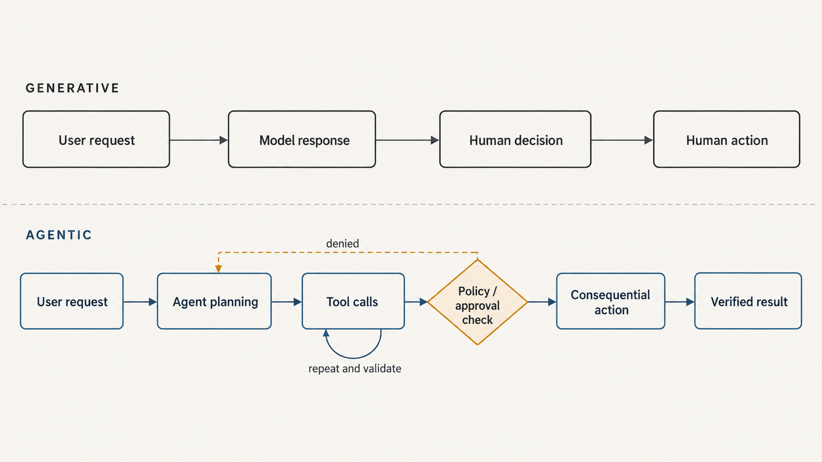
Generative AI produces something a person then acts on. Agentic AI takes the action itself.

That’s a working shorthand, not a strict definition. Plenty of generative products call tools, and plenty of agentic systems stop and wait for a person before anything consequential happens. The useful line is narrower: does the software hand you a recommendation, or does it change something in the world, such as a ticket, an account, a purchase order or a repository, before you look?

The agentic AI examples below make that line concrete. Each takes a real task, mostly from 2026 deployments, done both ways, and asks the same four things: who acts, where approval happens, roughly how many model calls it takes, and what goes wrong when it fails. The answers don’t always flatter the agentic version.

Key Takeaways
  • Speed claims are real but rarely like-for-like. Sophos says AI closes 52% of its security cases unaided, but its headline time saving compares an older human process with agent-handled cases.
  • Careful deployments constrain the agent, not the model. Kognitos runs approved procedures through a deterministic engine and pauses on exceptions.
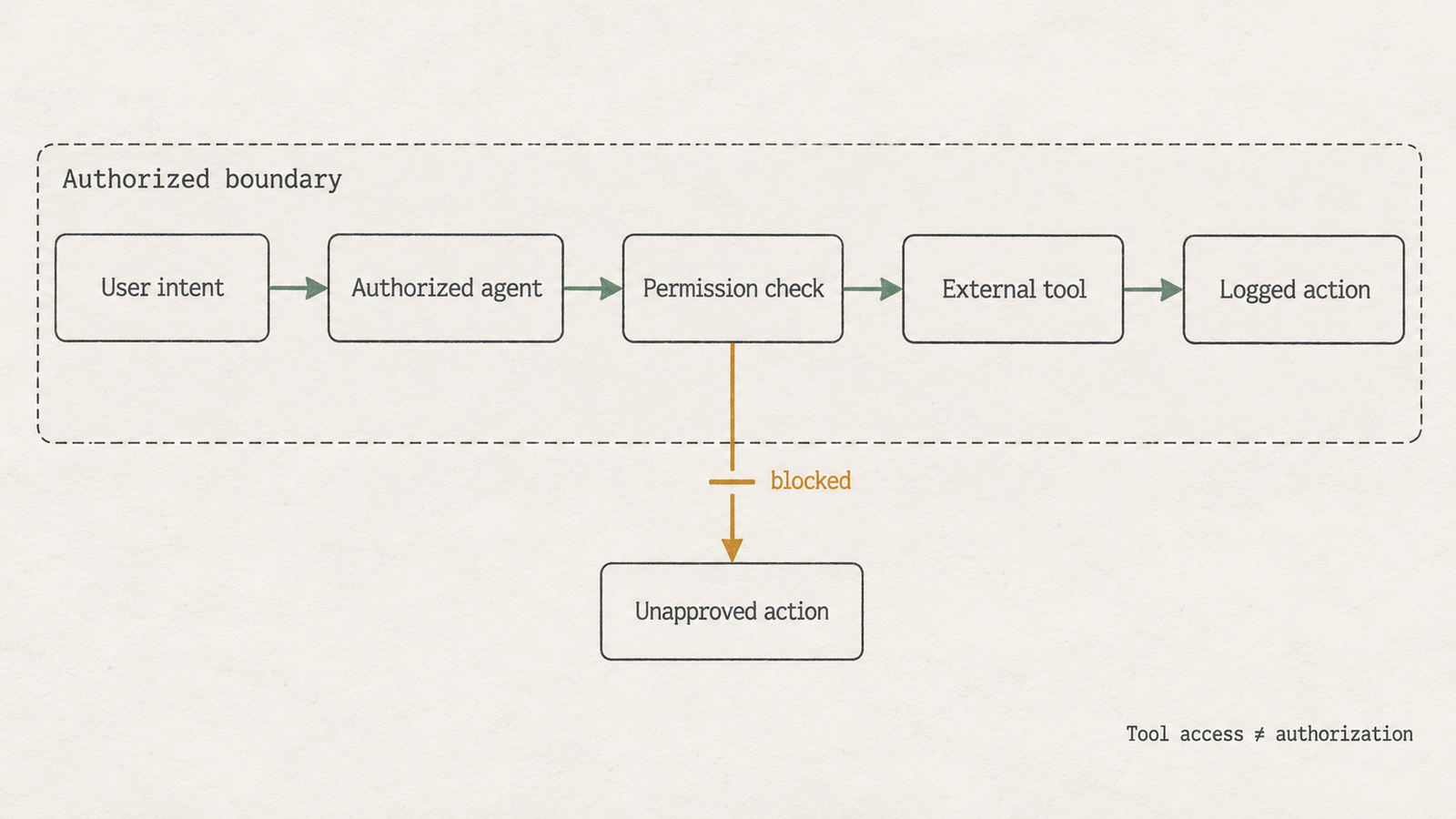
  • Access is not authorization. US banks found third-party agents inside customer accounts, mostly using passwords customers had handed over.
  • Identity and supervision are becoming product features. SK Telecom gives agents employee numbers and supervisors.
  • Agentic versions take more model calls per task, often ten times more in our illustrative ranges. That pays only where the action, not the advice, is the expensive part.

Quick Navigation


Part I: What separates agentic AI examples from generative ones

The difference sits in five places, and only one of them is the model.

Generative workflowAgentic workflow
AuthorityNone. It produces text, code or imagesDelegated. It can change records, send messages, spend money
Tool accessOptional, usually read-only (search, retrieval)Required, often with write access
Who executesA person, after reading the outputThe agent, through tools and APIs
Human approvalImplicit: nothing happens until someone actsExplicit: placed before consequential steps, or replaced by policy
Failure handlingA bad answer gets ignored or correctedA bad action has to be detected, stopped and often reversed

The last row carries the most weight. A wrong answer costs the reader’s time. A wrong action costs whatever it touched, plus the work of finding out it happened. That’s why most generative AI examples never need an audit trail, while the serious agentic deployments below invest in permissions, logs and pause points. Our earlier comparison of agentic and generative AI on cost, risk and control covers the architecture. This piece stays with the work.

agentic AI

Part II: Ten agentic AI examples, each shown two ways

Agentic AI examples where speed changes the workflow

1. Security operations: Sophos

Attackers don’t wait for a shift change, so security is where agent speed shows first. In a May 2026 release, Sophos said AI had closed 52% of its managed detection and response cases end to end over 12 months, inside boundaries “continuously calibrated by analysts”, with automated responses in 89 seconds. OpenAI has since headlined the work as a 96% cut in investigation time using its Daybreak program. TechInformed notes the comparison sets a roughly 38-minute average for the older, mostly human process against agent-handled cases, not matched cases.

  • Generative: a model summarises the alert and suggests containment. An analyst decides and isolates the host.
  • Agentic: the agent investigates, correlates telemetry and closes or contains the case.
  • Approval: “human-on-the-loop” for high-volume, well-bounded cases; “human-in-the-loop” for high-stakes ones.
  • Model calls (illustrative): one to three versus dozens.
  • Failure: a false negative closed fast looks exactly like a success. Neither company has published miss rates.
2. Coding: Claude Code

Coding agents are the best-documented case. Anthropic’s Claude Code documentation describes a tool that reads a codebase, edits files, runs commands such as test suites, commits and opens pull requests.

  • Generative: a chatbot writes a function. The developer pastes it in, runs the tests and fixes what breaks.
  • Agentic: the agent edits across files, runs the tests, fixes failures and opens a pull request.
  • Approval: by default it asks before edits and shell commands. Teams can deny commands such as git push, and the prompt-skipping mode is meant for isolated containers only. Merging stays behind branch protection and review.
  • Model calls (illustrative): one versus tens for a fix-and-verify loop.
  • Failure: the agent makes tests pass by weakening them. A reviewer who reads only the green checkmark won’t notice.
3. Research: multi-source investigation

Research agents automate reading the tenth source. Claude’s Research runs “multiple searches that build on each other”. OpenAI’s deep research documentation says its models can synthesize “hundreds of sources” over tens of minutes, with a max_tool_calls limit as the main cost control.

  • Generative: a model answers from memory, and the person checks sources.
  • Agentic: the agent searches, reads, discards weak sources, searches again and writes a cited report.
  • Approval: usually none mid-run.
  • Model calls (illustrative): one versus dozens to hundreds of tool calls.
  • Failure: a citation that doesn’t support its sentence. In a March 2025 Tow Center study, AI search tools cited news sources incorrectly in more than 60% of tests. A link proves a page exists, not that it says what the report claims.

Agentic AI examples that touch money

4. Personal finance: a subscription audit

Cisco president Jeetu Patel told Business Insider, as reported by Business Today, that a personal agent with access to his email flagged about $9,000 a year in subscriptions. It built a table of costs at his request. He picked two to cancel, and the agent cancelled them and sent confirmation emails, saving $1,000 to $1,200 a year for an agent costing $20 a month.

  • Generative: paste a statement into a chatbot, get a list, cancel each subscription yourself.
  • Agentic: the agent searches the inbox, builds the list and completes the cancellations you choose.
  • Approval: finding and recommending were automatic. Cancelling waited for Patel’s choice.
  • Model calls (illustrative): a handful versus tens.
  • Failure: cancelling the wrong plan. Patel’s agent found a duplicate $11.95 Dropbox plan; cancelling the original instead would have broken his storage.
5. Finance back office: Kognitos

Kognitos takes the opposite approach to free-roaming agents: its 21 October announcement offers 61 role-based “AI Employees”, from accounts payable to KYC, backed by 515 standard operating procedures. Models read documents, but a deterministic engine runs each approved procedure, and a case outside it pauses for a person.

  • Generative: a model summarises invoice matches, and an accountant posts the entries.
  • Agentic: the AI Employee matches the invoice and posts to the ERP under an approved procedure.
  • Approval: teams decide action by action what runs unasked. New procedures need a person’s sign-off.
  • Model calls (illustrative): a few for document reading either way. The procedure itself runs as code.
  • Failure: an exception nobody anticipated. Kognitos stops, which is slow but recoverable.
6. Laboratory procurement: Scientist.com

Scientist.com’s 22 October launch describes agents that read an uploaded experimental protocol, identify the services needed, match labs from more than 6,000 suppliers, compare proposals and turn the chosen one into a purchase order under the customer’s purchasing policies.

  • Generative: a model lists which assays to source, and a scientist emails labs for quotes.
  • Agentic: the agent finds suppliers, gathers proposals and prepares the order.
  • Approval: organisations “can” keep humans at supplier selection and financial commitments. The release doesn’t say they must.
  • Model calls (illustrative): a few versus tens.
  • Failure: a protocol misread at step one, such as the wrong sample volume, carried through to a valid-looking order.

Agentic AI examples where access becomes the product

7. Workforce management: SK Telecom

SK Telecom began giving AI agents employee numbers in June. Its first AI governance report, covered on 26 October, says each agent’s role, supervisor, status and performance are tracked. Higher-autonomy agents report to a team leader or executive, token use and work records are under review, and unnecessary agents are retired.

  • Generative: an employee uses a chatbot and answers for what they do with it.
  • Agentic: the agent works under its own identity, and a named supervisor answers for it.
  • Approval: human review tightens as autonomy rises.
  • Model calls: the point here is visibility, which is what token monitoring is for.
  • Failure: an orphaned agent still running after its owner moves on. An ID helps only if someone reads the logs; see why agents shouldn’t share a service account.
8. Banking: the failure case
agentic AI

On 22 October, Axios reported that major US banks had found third-party AI agents inside customer accounts. CBS’s follow-up says most cases involved customers giving their password to an agent the bank hadn’t vetted. Some activity “appeared” to exceed what the holder asked, including an agent that called a bank to file a complaint without first consulting the account holder. No losses were reported, and some banks are now blocking such agents.

  • Generative: a chatbot explains how to dispute a charge, and the customer calls the bank.
  • Agentic: an agent logs in as the customer, with the customer’s password but not the bank’s permission.
  • Approval: none the bank can see. That is the problem.
  • Model calls (illustrative): tens per session.
  • Failure: the bank can’t tell a customer’s agent from an attacker, which is why banks are moving toward read-only agent access.
9. Email: drafting versus sending

Microsoft Graph splits the line into two permissions: Mail.ReadWrite can create a draft, and sending needs Mail.Send. Google’s Gemini agent, announced on 8 October, ranks the inbox, can start email threads to arrange meetings, and logs every action to an audit trail attributed to the agent.

  • Generative: a model drafts a reply. You edit it and press send.
  • Agentic: the agent triages, drafts and, if it holds send permission, sends.
  • Approval: set by the permission. A draft-only agent can’t send, whatever it decides.
  • Model calls (illustrative): one per reply versus tens for a triage pass.
  • Failure: a confident reply to the wrong thread, or to a phishing email.
10. Computer use: GPT-6.1 Terra

OpenAI released GPT-6.1 Terra, a model built for computer use, on 26 October. The Next Web reports that in one of OpenAI’s own tests it turned architectural drawings into a 3D model. OpenAI hasn’t published details of that test, so treat it as a demonstration, not a deployment.

  • Generative: the model explains the CAD steps, and a drafter does them.
  • Agentic: the model operates the CAD application, clicking and typing from screenshots.
  • Approval: OpenAI’s computer-use guide tells developers to “ask for approval before making changes” and to use an isolated desktop, because “page content can influence the model”.
  • Model calls (illustrative): one versus dozens to hundreds of screenshot-and-act steps.
  • Failure: a misclick that silently changes a dimension, or hidden page instructions, the risk covered in our agent prompt injection testing analysis.

Part III: What the ten agentic AI examples reveal

Put the cases side by side and the interesting differences are about control, not intelligence.

CaseAuthority delegatedApproval boundaryReversible?Audit trail
SophosClose or contain casesAnalyst-set limitsMostlyNot described
Claude CodeEdit, run, open PRsPrompts or rules; humans mergeYes (git)Git history
ResearchRead, summariseNone mid-runYesCitations, unchecked
SubscriptionsCancel servicesUser picks eachPartlyConfirmation emails
KognitosPost to ERPPer action; exceptions pausePartlyRun journal
Scientist.comPrepare ordersOptional at spendPartlyProcurement system
SK TelecomVariesTightens with autonomyVariesPer-agent records
Bank agentsWhatever the password allowsNone the bank seesUncertainCan’t tell agent from person
EmailDraft, or sendThe permission grantedNot once sentSent folder, agent log
Computer useAnything on screenDeveloper-built stepsDepends on appScreenshots, if kept

Four patterns stand out.

  1. Reversibility decides where approval belongs. Code is easy to undo, so Claude Code can act freely and leave merging to people. A sent email or a cancelled subscription isn’t, so approval sits right before the action.
  2. Logs matter more as agents act faster. Kognitos, Google and SK Telecom all describe per-agent records. The bank case shows what happens when a log exists but can’t say who acted.
  3. Tool access sets the blast radius, and recovery depends on design. The email agent’s reach is one permission. The computer-use agent’s reach is the whole screen. Kognitos recovers from errors by stopping. Most others recover only when a person notices.
  4. Model calls multiply cost, and few vendors show it. The agentic versions run roughly ten to a hundred times more calls in these illustrative ranges, before retries. Only OpenAI’s max_tool_calls cap and SK Telecom’s token monitoring address cost visibility directly. That overhead is cheap next to an analyst’s half hour and expensive next to an answer someone would have checked anyway, as we worked through in when adding an agent stops paying for itself.

Part IV: When should a workflow become agentic?

Start with the action, not the model. A workflow is a good agent candidate when four things hold:

  1. The action is the bottleneck. If a person can act on advice in seconds, an assistant is enough.
  2. The action is bounded by permissions, not prompts.
  3. Mistakes are detectable and reversible, or the irreversible step sits behind a human or policy check.
  4. Someone owns the outcome: a named person reads the logs and can switch the agent off.

Keep a fixed, coded workflow when the steps never vary, such as a nightly reconciliation. Kognitos’s engine is effectively that, with a model reading the inputs. Use a generative assistant when judgment matters more than speed: a contract summary, a design review, a first draft.

Avoid agents where authority is borrowed rather than granted, as in the bank case. Avoid them, too, where one wrong action is costly and hard to spot, such as wire transfers or production deployments, unless a person approves each one. That agent can still save time. It just isn’t autonomous, and shouldn’t be sold as if it were.

The one-line test

Agency doesn’t reduce to one rule. Agents differ in how much they plan, which tools they hold and how often they ask. As a practical heuristic for any product calling itself agentic, though, one test works well:

If removing the human changes what happens next, it’s agentic.

Frequently asked questions

What are real-world agentic AI examples?

Documented 2026 examples include Sophos closing 52% of its security cases with AI, Kognitos’s finance “AI Employees”, Scientist.com’s procurement agents, and coding agents such as Claude Code that open pull requests. In each, software takes the action itself: closing a case, posting an entry, preparing an order.

How is agentic AI different from generative AI?

Generative AI produces content that a person reviews and acts on. Agentic AI uses tools to carry out actions itself, often over many steps and model calls. The practical differences are delegated authority, write access, and failure: a bad answer gets ignored, but a bad action has to be found and reversed.

Can generative AI perform actions?

Some generative products call tools, such as web search or a code interpreter, but they usually return results to a person rather than changing external systems. The line blurs when a chat assistant can also send email or edit files. At that point it’s behaving agentically, and its permissions matter more than its label.

Do agentic AI systems always need human approval?

No. Sophos says its AI closes about half of its cases without human intervention. Well-run systems place approval where actions are consequential or hard to undo, such as payments, sent messages and merges, and let reversible or low-risk steps run under policy limits.

Are agentic AI systems more expensive?

Per task, usually yes in model calls, because an agent plans, calls tools, checks results and retries. Whether that’s expensive depends on what it replaces. Dozens of model calls can cost less than a few minutes of an analyst’s time, but far more than a single answer a person would have checked anyway.

What is the biggest risk of autonomous AI agents?

Acting beyond intended authority. The October 2026 bank reports describe agents using customers’ passwords in ways banks hadn’t approved and, in some cases, customers apparently hadn’t either. Narrow permissions, separate agent identities, logs that attribute every action, and human approval for irreversible steps reduce that risk.


Keep reading

Anthropic IPO valuation

Anthropic IPO: The $895 Billion Question Behind Its Valuation

Last updated: 9 November 2026. Latest confirmed development: Anthropic’s amended S-1, filed on 2 November, still leaves the share count and the IPO price range …
Claude Opus vs Sonnet

Claude Opus vs Sonnet: What the 2026 Price Gap Actually Buys

Last verified: 8 November 2026. All prices are Anthropic’s standard first-party API rates in US dollars per million tokens. They aren’t Claude Pro or Max …
RSA-1024

Did AI Break RSA? What DeepMind Actually Found

Last verified: 8 November 2026. Both papers are unreviewed working papers, and no outside group has reproduced the results yet. No, AI did not break …
Model Distillation

Model Distillation Explained: When AI Learning Becomes Extraction

Last verified: 7 November 2026. Government and company claims are attributed throughout. None has been tested in court. A support team trains a small, cheap …

DeepSeek V4.1 Flash on a 12GB GPU

DeepSeek V4.1 Flash

Published 29 October 2026. Checked against ISTA-DASLab’s model card (updated 27 October), Strata’s documentation for version 0.2.7 and llama.cpp release b11870.

The 2-bit build of DeepSeek V4.1 Flash that runs on a 12GB graphics card is a 248.84GB set of files. That’s twenty times the card’s memory, and it is not a contradiction. You can run DeepSeek V4.1 Flash locally on a 12GB GPU because the card never holds the model. The GPU does part of the arithmetic, system RAM caches the experts used most often, and an NVMe SSD supplies the rest.

So the question worth asking isn’t whether 12GB of VRAM is enough. It’s whether the rest of the computer is. Strata, the open-source runtime behind the 12GB claim, documents a working setup with 46GB of system RAM and calls 64GB comfortable. Its developer measured between 4 and 11 tokens per second on 12GB cards, depending on the machine.

Quick answer
  1. Can it run? Yes, through Strata, on NVIDIA RTX 30, 40 or 50 series cards with 12GB or more, under Windows or Linux.
  2. What else you need: about 46GB of system RAM at minimum (64GB is Strata’s tested comfortable size), an NVMe SSD with roughly 245GB to 280GB free, and a modern CPU that will do much of the expert computation.
  3. Package size: 231.32GB to 265.83GB for the three ISTA-DASLab builds. Strata’s downloads are 239GB to 274GB because they add an 8GB draft model.
  4. The main limit: data movement. On 12GB cards, most of each token’s time goes to waiting on the SSD and CPU.
  5. Who should try it: people who want a frontier-scale open model offline, can accept a few tokens per second, and already own a machine with the RAM and disk.
Key Takeaways
  • 763 billion parameters isn’t the working size. Most of it is a 552-billion-parameter backbone and 196 billion parameters of Engram lookup tables, read a few rows at a time.
  • 248.84GB is a disk total, not a RAM requirement: a 138.24GB backbone plus a shared 110.60GB Engram file.
  • System RAM and the SSD matter as much as the GPU. Strata’s RAM expert cache ran about twice as fast as memory-mapping the files on the developer’s RTX 5070 machine.
  • “100% recovery” covers three benchmarks. Strata’s own test found the same build’s perplexity 15.5% higher on general text.
  • Strata’s 12GB default isn’t the full model. It routes each token to five of the model’s six experts unless you choose “Full quality”.
  • llama.cpp supports the model from release b11870.

Quick Navigation


What it takes to run DeepSeek V4.1 Flash locally on a 12GB GPU

Three numbers are easy to blur here, and they answer different questions.

Package size on disk is how much storage the files take: 248.84GB for the recommended IQ2_XXS build. Memory in use is what has to sit in VRAM and RAM while the model generates. Bandwidth is how fast the weights a token needs can reach whatever is computing it. A setup can pass the first two tests and still be slow on the third.

The architecture is what makes this possible. DeepSeek’s model card describes a mixture-of-experts (MoE) design: each MoE layer has 384 routed experts, small feed-forward networks, plus one shared expert. A router sends each token to six of the 384. DeepSeek puts the active parameters at 8 billion per token during prefill and 16 billion during decoding, out of 552 billion in the backbone. Most of the model sits idle for any given token.

The Engram component works differently again. It is 196 billion parameters of what DeepSeek calls “conditional memory”, accessed by token-based lookup rather than matrix multiplication. ISTA-DASLab’s card says the table is read one row per token. That’s why 110.60GB of it can stay on an SSD without hurting speed much.

The 763-billion headline figure comes from the Hugging Face metadata for the 1017 revision. The backbone and Engram add up to about 748 billion, and neither DeepSeek nor ISTA-DASLab explains the remaining 15 billion.

DeepSeek V4.1 Flash

The files you need to run DeepSeek V4.1 Flash locally

ISTA-DASLab, the Distributed Algorithms and Systems lab at the Institute of Science and Technology Austria, published three GGUF builds of DeepSeek-V4.1-Flash-1017, the 17 October revision. The method has two parts. GSQ chooses how each weight is rounded. RCO decides which quantization type each tensor gets so the total fits a size budget. Routed experts get between roughly 1.5 and 3.5 bits per weight. Dense tensors keep between about 5.5 and 8.5.

BuildBits per weightBackboneEngram fileCard totalStrata downloadReported quality
IQ1_M1.75120.72GB110.60GB231.32GB239GB98.7% of base task average (ISTA); perplexity +21% (Strata)
IQ2_XXS2.00138.24GB110.60GB248.84GB257GB100% of base task average (ISTA); perplexity +15.5% (Strata)
IQ2_XS2.25155.23GB110.60GB265.83GB274GB99.8% of base task average (ISTA); perplexity +7.3% (Strata)

The card total is the backbone plus the shared Engram file, in decimal gigabytes (10⁹ bytes). It excludes a 0.97GB vision projector. Strata’s download adds an 8GB draft model used for speculative decoding. Neither number is a measured runtime requirement.

The Engram file, stored in a 4.5-bit format called IQ4_NL, is identical across builds, so comparing them doesn’t mean downloading it twice. Strata recommends IQ2_XS for coding and agent work if disk allows: half the perplexity gap of IQ2_XXS, for 17GB more storage and slightly slower generation.

How Strata splits the model across GPU, RAM and SSD

Strata is an MIT-licensed local runtime maintained by a developer publishing as Niko1221. It added DeepSeek V4.1 Flash in version 0.2.4 on 24 October and was at 0.2.7 when this was written. Its DeepSeek engine, strata-dsv41, is a separate package ported from Project Maya’s MIT-licensed maya-ds4.

According to Strata’s DeepSeek guide and release notes, the work is split three ways. The GPU holds the dense weights and as many routed experts as fit, and computes them. A RAM expert store, which sizes itself to free memory when the engine starts, keeps the most-used experts in system RAM, and the CPU computes those. Experts that fit in neither are read from the model files on the SSD as they’re needed. A hot-expert profile ships with the engine, so the caches don’t start empty.

The Engram table is read “from RAM or SSD”. With 46GB to 64GB of RAM against a 138GB backbone, some disk reads during generation are unavoidable on a 12GB machine.

Strata’s 0.2.4 release notes compare this design with plain memory-mapping, where the operating system pages file data in on demand. On an RTX 5070 with 64GB of RAM, the expert store produced 4.3 to 4.9 tokens per second, against 1.8 to 2.2 for memory-mapping.

Two defaults matter for quality. The guide says context is set to 8,192 tokens, “the size it was checked at”, and --context raises it. On machines whose GPUs total 16GB or less, a “Faster” mode routes each token to five experts instead of the model’s six. The guide describes the quality change as “usually not noticeable”. Neither ISTA-DASLab’s benchmarks nor Strata’s perplexity figures say they used that mode, so “Full quality” (--experts 6, engine 0.1.50 or newer) is the setting that matches the published evidence.

DeepSeek V4.1 Flash

How fast DeepSeek V4.1 Flash runs locally

Strata’s README reports these figures, measured by its developer on version 0.2.5. UniverseBlend hasn’t reproduced them.

MachineSystem RAMOutput speedPrompt processing
RTX 5070 12GB, Ryzen 5 7600, 3.6GB/s NVMe64GB4–6 tokens/s231 tokens/s at 8K (0.2.4 notes)
RTX 3060 12GB46GB9–11 tokens/s149 tokens/s at 8K (0.2.4.1 notes)

The older RTX 3060 beating the RTX 5070 is a reminder that the GPU isn’t the main variable here. The project doesn’t explain the gap, and CPU, SSD and RAM configuration all differ between the two machines.

A back-of-envelope figure shows why storage dominates. If all 16 billion active parameters came off the SSD at about 2 bits each, every token would need roughly 4GB read. At 3.6GB per second, that’s about one token per second. That’s a pessimistic bound, because the dense weights stay on the GPU. Strata’s 4 to 11 tokens per second means caching is doing most of the work. A slower SSD, less RAM or a different mix of topics, which changes which experts are hot, pushes the system back toward that floor. Our earlier piece on the memory-bandwidth limits of AI chips explains the same constraint at data-centre scale.

Reasoning length matters as much as raw speed. Strata’s default thinking budget is 32,768 tokens. At 5 tokens per second, a fully used budget is about 1 hour 49 minutes before the answer starts. A 2,000-token reply alone takes about 6.7 minutes. Strata describes 4 to 8 tokens per second as usable for chat but slow for long agent runs, which is a fair summary.

Can your desktop run DeepSeek V4.1 Flash locally?

Work through these in order. The first failure tells you what to upgrade.

  1. GPU: an NVIDIA RTX 30, 40 or 50 series card with at least 12GB, on Windows or Linux. AMD support covers the Radeon AI PRO R9700 on Linux, and Strata’s README adds Ryzen AI Max “Strix Halo” on Windows. Macs aren’t supported.
  2. System RAM: 46GB is the smallest configuration Strata reports working, and 64GB is its tested comfortable size. The guide calls anything under about 40GB “untested and slow”. Setup warns if RAM is short but doesn’t stop.
  3. Free SSD space: 245GB to 280GB, depending on the build, on one drive.
  4. Storage type: NVMe. Strata’s test machine used a 3.6GB/s drive, and the guide warns that a slow disk “slows every word”. Avoid SATA SSDs and hard drives.
  5. CPU: a recent desktop processor, since it computes the experts that don’t fit on the GPU. Strata uses AVX-512 on Zen 4 and Zen 5.
  6. Power and cooling: GPU, CPU and SSD stay busy together for long stretches, and an NVMe drive without a heatsink may throttle.
  7. Patience: a 250GB download, a load of several minutes, and replies measured in minutes.

These are the configurations Strata’s developer reports testing, not universal minimums.

Why the three-benchmark result needs context

ISTA-DASLab reports that IQ2_XXS matches the FP8/FP4 base model on all three tasks it measured, at reasoning effort 50:

VariantAIME25GPQA-DiamondLiveCodeBench v6Task average
Base model100.0090.9189.7193.54
IQ2_XXS (2.00 bpw)100.0090.9189.7193.54

The result comes from the team that made the quantization, on competition maths, graduate science and coding problems. “100% recovery” means those three scores were identical, not that the 2-bit build keeps every capability. Nothing here tests long-context recall, multilingual writing, tool use or image input. And with the base model already at 100 on AIME25, that benchmark can only register a loss.

Strata’s own measurement shows why that matters. On 4,995 text positions, the IQ2_XXS build’s perplexity, a measure of how well a model predicts text, was 15.5% higher than the original’s. That’s a different test from ISTA-DASLab’s, and it isn’t evidence that answers are 15.5% worse. It does show that a build can match on three reasoning benchmarks and still differ measurably elsewhere. The IQ1_M build’s perplexity on plain English prose was 53% higher.

For an independent view of the full model, Artificial Analysis gives DeepSeek V4.1 Flash 1017 at maximum reasoning effort a score of 32 on its Intelligence Index v5.0, which combines nine evaluations. That number is on v5.0’s scale and can’t be compared with scores from the older v4 index. It also measures DeepSeek’s hosted model, not a 2-bit local build. Epoch AI’s Capabilities Index is a separate evaluation: it lists 156 for the original September release. As we’ve argued in why benchmark scores don’t transfer to your workload, the useful test is your own tasks on your own build.

Running DeepSeek V4.1 Flash locally with llama.cpp

Standard llama.cpp support arrived recently. Release b11870, published as a pre-release on 25 October, adds the deepseek41 architecture and Engram handling. ISTA-DASLab’s card says its files have used the current layout since 27 October. Copies downloaded before then need a local conversion with the convert_ds41_upstream.py script.

The card also notes that llama.cpp’s default lazy mode memory-maps tensors over 4GiB, so the Engram file needs neither VRAM nor RAM. Strata’s RAM expert store and hot-expert profiles are its own additions, and in Strata’s comparison plain memory-mapping ran at roughly half the speed. On a 12GB card, expect llama.cpp to work but not to match Strata’s figures without tuning. We found no published like-for-like comparison of the two.

Is it worth the effort to run DeepSeek V4.1 Flash locally?

That depends on what you need the model for.

  • The case for local: offline use, data that can’t leave the machine, and experimenting with a frontier-scale open model at no per-token cost. The base model and ISTA-DASLab’s files are MIT-licensed, which permits commercial use.
  • The case for the API: price and speed. Artificial Analysis lists DeepSeek’s API at $0.30 per million input tokens and $1.20 per million output tokens, at about 184 output tokens per second. Generating one million output tokens locally at 5 tokens per second takes more than 55 hours of continuous running, a job the API would bill at $1.20.

Local isn’t automatically private either: downloads, engine updates and connected tools still touch the network. For coding agents, the API wins on throughput. For occasional private questions on hardware you already own, local is a reasonable choice. Our comparison of Chinese open-weight models covers the licensing terms and the US federal restrictions on DeepSeek products.

What the 12GB claim really tells us

A 12GB card is the cheapest part of this setup. What lets you run DeepSeek V4.1 Flash locally is a runtime that treats VRAM, RAM and an NVMe drive as one memory hierarchy, plus the 46GB to 64GB of RAM and 250GB of fast storage that hierarchy needs.

The headline is accurate, and it measures the wrong part of the computer. Check your RAM and your SSD first. Then decide whether a few tokens per second fits the work you have in mind.

Frequently asked questions

Can you run DeepSeek V4.1 Flash on a 12GB GPU?

Yes, with Strata, on an NVIDIA RTX 30, 40 or 50 series card with at least 12GB, under Windows or Linux. The GPU holds only part of the model. The rest is cached in system RAM and read from an NVMe SSD, so the card alone doesn’t decide whether the setup works.

How much RAM do you need to run DeepSeek V4.1 Flash locally?

Strata reports a working setup with 46GB and calls 64GB its tested comfortable size. Below about 40GB is untested and, in the developer’s words, slow. More RAM lets Strata keep more experts cached, which reduces SSD reads and raises speed.

Does the 248.84GB model size mean you need 248.84GB of RAM?

No. 248.84GB is the disk size of the IQ2_XXS build: a 138.24GB backbone plus a 110.60GB Engram lookup file. The Engram file is read a row at a time, and Strata caches only the most-used experts in RAM. The rest stays on the SSD until needed.

Can DeepSeek V4.1 Flash run with standard llama.cpp?

Yes, from release b11870 (25 October 2026), which adds the deepseek41 architecture. ISTA-DASLab’s files have matched that layout since 27 October; earlier downloads need converting first. By default llama.cpp memory-maps large tensors, and Strata measured memory-mapping at roughly half the speed of its own RAM expert store.

What is the difference between IQ1_M, IQ2_XXS and IQ2_XS?

They are 1.75, 2.00 and 2.25 bits per weight on average, with backbones of 120.72GB, 138.24GB and 155.23GB, sharing one 110.60GB Engram file. More bits mean better fidelity: Strata measured perplexity increases of 21%, 15.5% and 7.3% over the original. Smaller builds suit tight disks.

Does the 2-bit quantized model retain 100% of the original model’s performance?

Only on the three benchmarks its makers report: AIME25, GPQA-Diamond and LiveCodeBench v6, where IQ2_XXS matched the base model’s scores. Strata’s perplexity test found a 15.5% gap on general text. Treat “100% recovery” as a statement about those three tasks.

Will DeepSeek V4.1 Flash run quickly on an ordinary desktop?

Not by API standards. Strata’s developer measured 4 to 6 tokens per second on an RTX 5070 with 64GB of RAM, and 9 to 11 on an RTX 3060 with 46GB. That’s workable for chat, but long reasoning traces and agent loops can take many minutes per answer.

Is running DeepSeek locally better than using an API?

For offline work or restricted data on hardware you already own, it can be. For throughput, DeepSeek’s API is far faster, at about 184 tokens per second, and it charges $1.20 per million output tokens. Local use also isn’t automatically private: setup, updates and connected tools still use the network.


Keep reading

Anthropic IPO valuation

Anthropic IPO: The $895 Billion Question Behind Its Valuation

Last updated: 9 November 2026. Latest confirmed development: Anthropic’s amended S-1, filed on 2 November, still leaves the share count and the IPO price range …
Claude Opus vs Sonnet

Claude Opus vs Sonnet: What the 2026 Price Gap Actually Buys

Last verified: 8 November 2026. All prices are Anthropic’s standard first-party API rates in US dollars per million tokens. They aren’t Claude Pro or Max …
RSA-1024

Did AI Break RSA? What DeepMind Actually Found
Last verified: 8 November 2026. Both papers are unreviewed working papers, and no outside group has reproduced the results yet. No, AI did not break …
Model Distillation

Model Distillation Explained: When AI Learning Becomes Extraction

Last verified: 7 November 2026. Government and company claims are attributed throughout. None has been tested in court. A support team trains a small, cheap …

LLM Cost per Task: How to Calculate the Real API Cost

LLM cost

Prices checked 28 October 2026: standard (pay-as-you-go) API tier, US dollars per million tokens, from each provider’s official pricing page unless stated otherwise.

Kimi K3.1 Pro costs half as much per token as Claude Opus 5.5: $2 per million input tokens and $10 per million output tokens, against $4 and $20. On Artificial Analysis’s Intelligence Index runs, Kimi still cost more per task: $2.11 against $1.82 for Opus 5.5 at High effort. It produced 55,000 output tokens per task to Opus’s 36,000.

That’s the mistake a price table invites. A per-token rate tells you what one unit of text costs. It doesn’t tell you how many units a model will spend on your job, or how often the job comes back usable. LLM cost per task captures both.

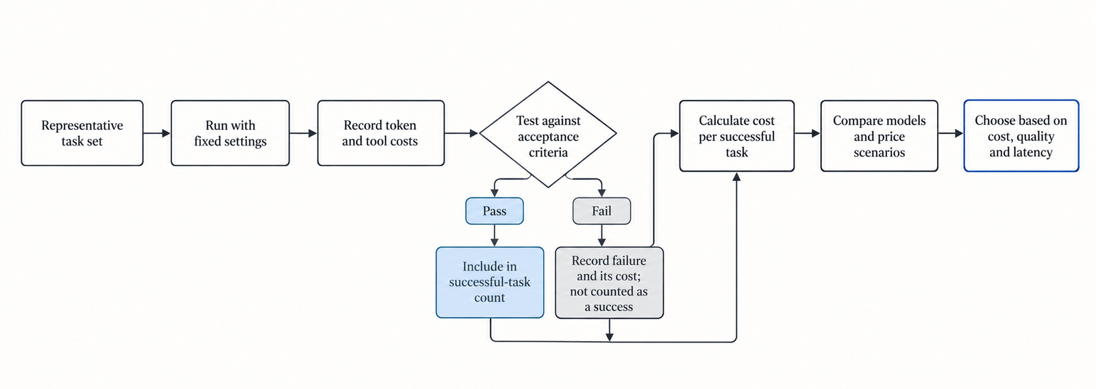
LLM cost per task is the total API spend on every attempt at a set of tasks, divided by the number of attempts that met your acceptance criteria.

The rest of this article is about calculating that number correctly, and about knowing when to trust it.

Key Takeaways
  • Price per token and cost per task can rank models in opposite orders. Kimi K3.1 Pro is half Opus 5.5’s per-token price but cost about 16% more per Artificial Analysis task.
  • Reasoning tokens are billed as output by OpenAI, Anthropic and Google, even when you never see them. Anthropic also bills earlier turns’ thinking as input on its newest models.
  • Caching can swing the bill several-fold. In one public test, a broken cache made a single run cost $17.60 instead of $2.62.
  • Divide by successes, not attempts. Failed runs cost money and produce nothing.
  • Twenty runs can’t separate close results. An 80% and a 65% pass rate from 20 runs each have overlapping confidence intervals.
  • Price changes can settle a close call. One developer test found Gemini 4 Argon roughly level with Opus 5.5 per successful fix. At Argon’s December 1 prices, it would cost about twice as much.

Quick Navigation


The LLM cost per task formula

For one attempt, the API cost is the sum of each token category times its rate, with token counts converted to millions:

Attempt cost = (fresh input tokens  ÷ 1,000,000 × fresh-input rate)
             + (cache-read tokens   ÷ 1,000,000 × cache-read rate)
             + (cache-write tokens  ÷ 1,000,000 × cache-write rate)
             + (billable output     ÷ 1,000,000 × output rate)
             + per-call charges (web search, code containers, grounding)

Then, across a test set:

LLM cost per successful task = sum of all attempt costs ÷ number of successful attempts
LLM cost

Each line has its own billing rules, and they differ by provider. This is the buyer’s cost. What it costs a provider to serve those tokens, and its margin, is a separate question, covered in what inference actually costs per token.

What each line costs at OpenAI, Anthropic and Google
Line itemOpenAI (GPT-5.6 and later)Anthropic (Claude 5.5 models)Google (Gemini 4 Argon)
Fresh inputList rateList rateList rate
Cache read0.1× input; 0.05× on GPT-6.1 Sol and Terra0.1× input; 0.05× on Opus 5.5 and Sonnet 5.5$0.10 per million (0.05× input)
Cache write1.25× input (30-minute) or 2.5× (12-hour)1.25× input (5-minute) or 2× (1-hour)No separate charge listed; caching is implicit only
Reasoning tokensBilled as outputBilled as output, including when thinking text is hiddenBilled as output (“incl. thinking”)
Search tools$10 per 1,000 web searches$10 per 1,000 web searches$14 per 1,000 grounded queries after 5,000 free a month

Sources: OpenAI pricing and prompt caching; Anthropic pricing and prompt caching; Gemini API pricing.

Two details catch people out. Anthropic’s thinking defaults to a display mode of “omitted” on Opus 5.5 and Sonnet 5.5, but its thinking documentation is explicit: “You’re still charged for the full thinking tokens. Omitting reduces latency, not cost.” On those models, previous turns’ thinking blocks also stay in context and are billed as input, so a long agent session pays for old reasoning again on every turn.

Reading usage fields without double-counting

A common error in home-made calculators is adding a field that already contains another one.

  • Anthropic: input_tokens counts only the tokens after the last cache breakpoint. Total input is cache_read_input_tokens + cache_creation_input_tokens + input_tokens, and each part takes its own rate.
  • OpenAI: cached_tokens excludes tokens charged as writes, which appear in cache_write_tokens. Reasoning tokens sit inside output_tokens, under output_tokens_details.reasoning_tokens. Don’t add them again.
  • Truncated responses: with reasoning models, a request that hits its output limit can bill input and reasoning tokens and return no visible answer, as OpenAI’s reasoning guide warns. That attempt still counts toward the cost.

Then reconcile your summed usage against the provider’s invoice for the same period. In July 2026, developers on OpenAI’s forum reported that GPT-5.6 output-token counts were several times higher than the text actually generated. OpenAI didn’t publicly confirm a defect in that thread. Whatever happened there, the invoice is the figure your finance team will pay.

From cost per attempt to LLM cost per successful task

The numerator is everything you paid to get results. That includes failed attempts, automatic retries, intermediate calls inside an agent loop, any model you use as a judge and per-call tool fees. Count each API call once, at the moment it happens. If your harness logs both an agent step and its parent run, sum only one of them.

The denominator is the number of attempts that passed a fixed acceptance test, written before the run. “The tests pass” is a test. “The output looked fine” is not. The same criteria must apply to every model, or the division compares different jobs.

There are two valid ways to define a task:

  • Independent attempts. Each run is scored on its own, which is what most benchmark-style comparisons do.
  • Tasks with a retry policy. A task succeeds if any attempt within, say, three tries passes. Then the cost per task is all spend divided by tasks completed. That matches production better, but pick one definition and use it for every model.

API cost is not the whole bill. Human review, retrieval infrastructure, observability and sandboxes belong in a fully loaded cost per task whenever models differ in how much of that work they create. A model whose failures are obvious and cheap to discard can beat one whose failures look plausible and need a reviewer to catch.

A public test: 20 runs, four models

On 14 October 2026, a developer writing at paddo.dev replayed six merged changes from a production monorepo against four models. Each model got 20 runs (three or four per change) at medium effort in the Claude Code harness. Gemini 4 Argon was routed through OpenRouter. A run passed if the tests that shipped with the original fix passed. Costs were calculated at list prices.

ModelRunsPassing runsTotal costCost per runCost per passing run
Gemini 4 Argon2016$57.68$2.88$3.61
Claude Opus 5.52013$45.81$2.29$3.52
Claude Sonnet 5.52011$11.76$0.59$1.07
GPT-6.1 Sol2011$6.73$0.34$0.61

The totals and pass counts come from the post. The last two columns are our arithmetic, and they check: $57.68 ÷ 16 = $3.605, and $45.81 ÷ 13 = $3.524.

Argon and Opus are close, nine cents apart per passing run. Argon’s per-token prices matched Sonnet 5.5’s at the time ($2 input, $10 output), yet it cost five times as much as Sonnet per run. It wrote 1.37 million output tokens across the 20 runs, 2.8 times as many as Opus.

GPT-6.1 Sol had the lowest cost per passing run, but the post also records five Sol runs that broke a previously passing test, against none for the others. It doesn’t say whether those runs are among Sol’s 11 passes. If “breaks nothing” is part of your acceptance test, Sol’s denominator may shrink, which is why the test has to be written down before anyone divides.

How much a 20-run test can tell you

Not much, at the margin. A 95% Wilson confidence interval on 16 passes out of 20 is about 58% to 92%; for 13 out of 20, about 43% to 82%. The ranges overlap heavily, so a rerun could reverse the order. And six changes from one codebase, with correlated runs on each change, say little about a different stack.

What the December repricing does

Google’s pricing page doubles every Argon token rate on 1 December 2026: input from $2 to $4, cached input from $0.10 to $0.20, output from $10 to $20. If the runs used identical tokens, Argon’s total would become $115.36, or $7.21 per passing run, about twice Opus’s $3.52. We covered the change itself in Gemini 4 Argon pricing doubles Dec 1.

A simple break-even check shows how far the decision moves. One model is cheaper per success than another when its pass rate exceeds the other’s pass rate multiplied by the ratio of their per-attempt costs. Before December, Argon needed a pass rate above 65% × 1.26 ≈ 82% to beat Opus; it scored 80%. After December, it would need 65% × 2.52 ≈ 164%, which is impossible. Even at the bottom of Opus’s confidence interval, Argon would lose. On this test, the price change settles a question the sample size couldn’t.

How caching and reasoning change LLM cost per task

The same post found a stark caching failure. The first Argon run cost $17.60 because it read 8.4 million input tokens and only 59,000 came from cache. The harness inserted system messages that changed the prompt prefix on every call, so Gemini’s implicit cache never matched. After a fix, the same run cost $2.62, with 94% of input served from cache.

The second example is illustrative. The token counts and pass rates are assumptions, not measurements of any real model. Two models attempt the same agent task:

  • Model X: $1 input, $0.05 cache read, $1.25 cache write, $5 output, per million tokens. Pass rate 60%.
  • Model Y: $4 input, $0.20 cache read, $5 cache write, $20 output. Pass rate 85%.
  • Each attempt sends 300,000 input tokens over its turns. When caching works, 270,000 are cache reads and 30,000 are cache writes.
  • Model Y produces 20,000 output tokens per attempt, including reasoning. Model X produces 60,000.
ScenarioCost per attemptPass rateCost per successful task
Model X, cache broken (all 300,000 input tokens fresh)$0.60060%$1.00
Model X, cache working$0.35160%$0.585
Model X, cache working, reasoning doubles to 120,000 output tokens$0.65160%$1.085
Model Y, cache working$0.60485%$0.711

The calculation for the second row: 270,000 × $0.05 + 30,000 × $1.25 + 60,000 × $5, each divided by one million, gives $0.0135 + $0.0375 + $0.30 = $0.351. Dividing by 0.60 gives $0.585.

LLM cost

With caching working, the cheaper model wins. Break the cache, or let it reason twice as long, and the expensive model wins instead. Neither change shows up in a price table.

What published comparisons actually measured

Before using a published cost-per-task figure, check the effort setting, what counted as a task, and whether success was part of the number.

  • Effort settings. Put Gemini 4 Argon’s 36,000 reasoning tokens per task next to Opus 5.5’s 84,000, and Argon looks far leaner. Both figures appear on Artificial Analysis, but they come from different settings: Argon at High effort and Opus 5.5 at Max. At matched High effort, the comparison reverses: Argon used 36,000 reasoning tokens per task to Opus’s 18,000, and 62,000 output tokens in total to Opus’s 36,000. Argon still cost less per task, $1.62 against $1.82, because its tokens were half the price at the time.
  • Vendor claims. OpenAI launched GPT-6.1 Terra on 26 October at $1 input and $5 output. DataCamp’s write-up of the announcement says that at max effort Terra is over three times as token-efficient as Opus 5.5 and a quarter of the price per token, and it puts the combined effect at “9x lower cost per task”, attributed to OpenAI. No benchmark is named, and we couldn’t open OpenAI’s post to check. Three times the efficiency at a quarter of the price would multiply to about 12 times, not 9, so the figure depends on a token breakdown that hasn’t been published. Treat it as a vendor claim to test, not a result.
  • Cost per task is not cost per success. Artificial Analysis computes cost per task from token counts at list prices. It doesn’t divide by how many answers were right. A model that is cheaper per task but scores lower may still cost more per correct answer. As we argued in why benchmark scores don’t transfer to your workload, these numbers are good for building a shortlist, not for making the final decision.

How to measure LLM cost per task on your own workload

  1. Pick 30 to 50 real tasks from production traffic, covering easy, typical and hard cases. More tasks beat more runs of the same task.
  2. Write the acceptance test first: unit tests, a schema check or a fixed-judge rubric, identical for every model.
  3. Fix the configuration: prompts, tools, effort setting, context limits and retry policy.
  4. Log raw usage for every call, including retries and sub-agents, with each token field stored separately.
  5. Price the logs offline against a dated copy of each pricing page, so you can reprice them when rates change.
  6. Check cache hit rates per model. A low rate in a repetitive session usually means the prompt prefix changes between calls.
  7. Reconcile with the invoice for the test window.
  8. Report ranges: pass rate with a confidence interval, cost per attempt, cost per successful task and latency.

Run at least two attempts per task. That shows whether failures are random or the same task fails every time.

A decision rule for LLM cost per task

Compare models on cost per successful task, after deciding what a success is worth. Then apply three checks.

  • If the confidence intervals on pass rate overlap, treat the models as tied on quality and choose on cost per attempt, latency and operational fit.
  • If one model’s cost per attempt is k times another’s, it needs a pass rate more than k times higher to win. When that would take a pass rate above 100%, stop testing.
  • If a success is worth far more than the API cost, as with a merged fix that saves an engineer an hour, pass rate and reviewer time outweigh token prices. Optimise for the fewest failures, then for cost.

Per-token prices still have a job. They tell you where to look first. LLM cost per task tells you what you’ll actually pay.

Frequently asked questions

What is LLM cost per task?

It is the total API spend on all attempts at a set of tasks, divided by the number of attempts that met a fixed acceptance test. Failed attempts, retries, intermediate agent calls and judge-model calls stay in the total, because you paid for them. A broader, fully loaded version adds review time and infrastructure.

How do I calculate LLM API cost for one request?

Multiply each token category by its rate per million tokens: fresh input, cache reads, cache writes and output, including reasoning. Then add per-call tool fees such as web search. Take the counts from the response’s usage object, and check that one field doesn’t already include another before adding them.

Are reasoning tokens billed?

Yes. OpenAI, Anthropic and Google bill reasoning or thinking tokens at the output rate, even when the reasoning text isn’t returned. On Anthropic’s Opus 5.5 and Sonnet 5.5, previous turns’ thinking blocks are also billed as input when they stay in the conversation.

How much does prompt caching save?

Cache reads cost between 5% and 10% of the input rate at OpenAI, Anthropic and Google for current models. OpenAI and Anthropic charge 1.25 times the input rate or more to write to the cache. Savings depend on how much of each request repeats an earlier prefix, so measure the hit rate rather than assuming it.

Is the cheapest model per token ever the cheapest per task?

Often, yes. On Artificial Analysis’s figures, Gemini 4 Argon at High effort cost less per task than Opus 5.5 at High, while its tokens were half the price. The ranking flips when the cheaper model uses many more tokens, misses the cache or fails more often. Only measurement on your own tasks tells you which case you’re in.


Keep reading

Anthropic IPO valuation

Anthropic IPO: The $895 Billion Question Behind Its Valuation

Last updated: 9 November 2026. Latest confirmed development: Anthropic’s amended S-1, filed on 2 November, still leaves the share count and the IPO price range …
Claude Opus vs Sonnet

Claude Opus vs Sonnet: What the 2026 Price Gap Actually Buys

Last verified: 8 November 2026. All prices are Anthropic’s standard first-party API rates in US dollars per million tokens. They aren’t Claude Pro or Max …
RSA-1024

Did AI Break RSA? What DeepMind Actually Found
Last verified: 8 November 2026. Both papers are unreviewed working papers, and no outside group has reproduced the results yet. No, AI did not break …
Model Distillation

Model Distillation Explained: When AI Learning Becomes Extraction

Last verified: 7 November 2026. Government and company claims are attributed throughout. None has been tested in court. A support team trains a small, cheap …

SpaceX’s $40B GPU Lease: The Customer Sets the Price

SpaceX GPU

Published 28 October 2026. This is a developing financing story. As of publication, SpaceX had signed a binding commitment letter (24 October), but the master finance lease hadn’t been signed, the fixed rate hadn’t been set, and the deal hadn’t closed. We will update this article when SpaceX discloses pricing or closing.

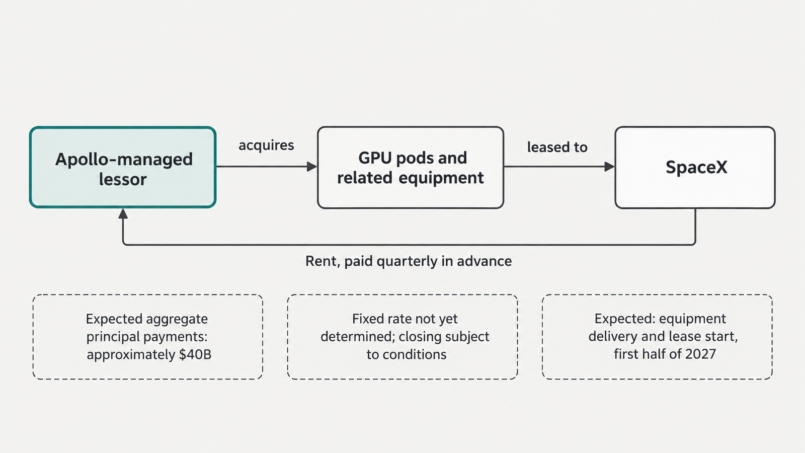
SpaceX announced on 26 October that it had secured “the largest committed GPU financing”: roughly $40 billion of Nvidia Vera Rubin equipment, to be bought by an Apollo-managed entity and leased to SpaceX. The Form 8-K filed the same day is more careful. It describes a binding commitment letter signed on 24 October, a lease that has not yet been signed, and a fixed rate that will be set “at pricing.”

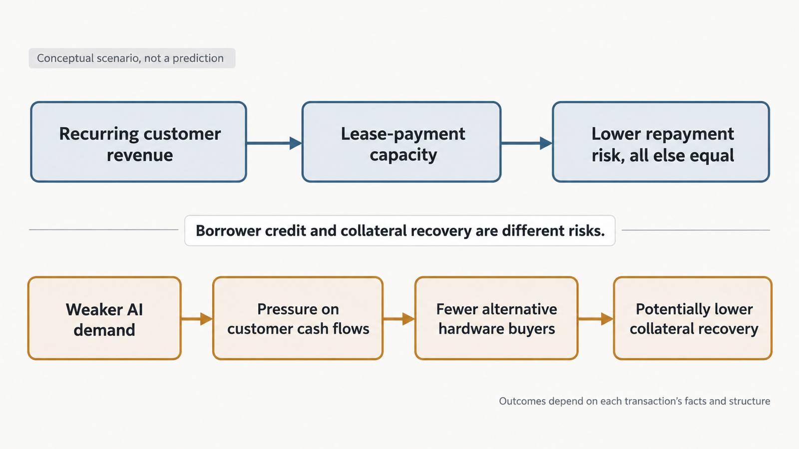
That missing rate is the most interesting part of the deal. In October, CoreWeave’s unsecured bonds traded at yields near 15%. Earlier in the year, the same company’s best-protected GPU loan carried a fixed rate of about 5.9%. Both are claims on one company’s GPU business. The difference came from who was expected to pay. SpaceX GPU financing will be priced by the same logic, and the documents suggest the investors are underwriting SpaceX far more than they are underwriting the chips.

Key Takeaways
  • Committed, not closed or priced. SpaceX signed a binding commitment letter on 24 October. The fixed rate, the master lease and closing come later, with closing expected before the end of 2026.
  • $40 billion is principal only. Interest and ongoing costs come on top. On illustrative assumptions, each percentage point on the rate adds roughly $1 billion of interest.
  • Rent repays the full hardware cost. Each quarterly payment covers one-twentieth of a tranche’s cost, so investors depend on SpaceX paying far more than on what used GPUs fetch.
  • SpaceX’s contracts end before the lease does. Only about 6% of its $63 billion backlog falls more than three years out. The lease runs to roughly 2032.
  • CoreWeave shows the customer setting the price. Its contract-backed, A3-rated GPU loan carried about 5.9% fixed. Its unsecured notes yielded near 15%. The instruments differ, so the gap reflects structure, not chips.
  • SpaceX’s earlier GPU leases look costlier than its bonds. Our estimate from its 10-Q puts the Valor lease debt at about 10.7% a year, against 5.35% to 6.65% coupons on its unsecured bonds.

Quick Navigation


How the SpaceX GPU financing actually works

The 8-K describes a lessor “managed by Apollo Global Management” that will acquire “graphics processing unit pods and related equipment” and lease them to SpaceX for use at data centres SpaceX selects. Apollo and Goldman Sachs lead the financing parties, with Goldman as sole structuring agent. Funds managed by BlackRock, Goldman Sachs Asset Management and KKR-advised accounts made anchor commitments.

The investors won’t hold a single loan. Bloomberg reported that the debt will take the form of private bonds issued by an entity that sits off SpaceX’s balance sheet. Pimco bought about $4 billion of an “A2” tranche that sits between more senior and more junior slices, according to Bloomberg’s sources. So the risk is layered before it reaches anyone’s portfolio.

The rent formula is the most revealing disclosure. Equipment arrives in tranches, and each tranche gets its own lease schedule of roughly five to five and a quarter years. Rent is paid quarterly in advance and “will generally consist of” one-twentieth of the tranche’s financed cost, plus a fixed-rate charge on the outstanding balance, plus certain ongoing costs.

Twenty payments of one-twentieth each return the full cost of the equipment. The lessor is counting on SpaceX’s payments, not on selling used Rubin racks in 2032. The 8-K is silent on end-of-term ownership, purchase options, guarantees and prepayment. Elon Musk called it on X “primarily callable debt”, but the filing describes no call feature.

The issuing entity may sit off SpaceX’s balance sheet, but the lease won’t. Under US accounting rules, a lessee records a finance lease as a liability once it commences.

SpaceX GPU
What the $40 billion does and doesn’t include

SpaceX “expects aggregate principal payments under the lease schedules over their respective terms to total approximately $40 billion.” That is the equipment cost being financed. The fixed-rate charge and the ongoing costs come on top, and neither has a published figure yet.

The scale matters. SpaceX reported $38.8 billion of long-term debt and capital lease obligations at 30 September in its third-quarter Form 10-Q. Once every tranche has commenced, principal alone runs to about $2 billion a quarter. For context, SpaceX generated $13.1 billion of operating cash flow in the first nine months of 2026 and held $89.9 billion of cash and marketable securities at quarter-end.

Four dates that are easy to confuse
MilestoneDateStatus
Commitment letter signed24 October 2026Done
Announcement and 8-K26 October 2026Done
Pricing (fixed rate set)Before the master lease is signedNot yet disclosed
Master lease signed and deal closedExpected before end of 2026Subject to unspecified conditions
Lease schedules beginOn delivery, expected first half of 2027Expected

Musk said on 25 October that the financing had closed. The company’s own filing, made a day later, does not say that. Where the two differ, this article follows the filing.

Whose credit backs SpaceX GPU financing

SpaceX has investment-grade ratings: Baa1 from Moody’s, BBB+ from Fitch and BBB from S&P, all with stable outlooks, according to Reuters on 18 June. Musk’s claim that “we’re investment grade and have Starlink & launch revenue” is accurate on the first point. Reuters also reported that S&P viewed the AI segment as the uncertain part, because of its capital needs and competition.

Bond investors have been less generous than the agencies. A Bloomberg Opinion column in July calculated that SpaceX’s average spread over Treasuries was slightly wider than the average for BB-rated, sub-investment-grade debt. On 21 October, the spread on SpaceX’s 6.6% notes due 2046 widened to 2.64 percentage points, and its five-year credit default swaps were near record highs, according to Bloomberg and ICE data relayed by Seoul Economic Daily.

These four measures answer different questions. A rating is an agency’s opinion of default risk. Musk’s description is an issuer’s claim. A bond’s yield is what investors pay today for an existing security with its own maturity and liquidity. The lease rate will be a negotiated price for a new, tranched instrument. None of them substitutes for the others.

The operating picture is strong but concentrated. Third-quarter revenue was $14.6 billion: $7.56 billion from the Super Intelligence (SI) segment, $5.25 billion from Starlink and $1.77 billion from launch. One SI customer supplied 34.5% of it. Nine-month capital spending of $48.1 billion far exceeded operating cash flow. SpaceX’s CFO cites payback periods under a year on SI infrastructure, without publishing the calculation.

A backlog that ends before the lease does

SpaceX reported a backlog of $63.0 billion at 30 September. It expects 67% of that to be recognised within a year, 27% in one to three years and 6% after that. Six per cent is about $3.8 billion. The lease payments, by contrast, run from 2027 to roughly 2032.

The contracts are also shorter than they look. Google’s agreement to pay $920 million a month runs to June 2029, but either side can end it on 90 days’ notice after 31 December 2026, TechCrunch reported from SpaceX’s filing. Anthropic’s $1.25 billion-a-month Colossus 1 agreement runs through 2029.

So the later years of rent are not covered by any contract SpaceX has disclosed. Investors are lending against SpaceX’s ability to keep selling compute, and behind that, against Starlink and launch. That is the opposite of how CoreWeave structures its cheapest debt.

CoreWeave: one GPU business, two prices

CoreWeave is the cleanest test of the idea that the customer, not the hardware, sets the price of GPU debt. The company borrows in two very different ways, and the price gap between them is wide.

The first is the delayed-draw term loan, or DDTL, raised inside a special-purpose subsidiary. CoreWeave’s March 2026 overview of DDTL 4.0 describes an $8.5 billion facility priced at SOFR plus 2.25 percentage points, with a fixed tranche at about 5.9%. Moody’s rated it A3. Lenders hold a first-priority claim on the equipment, the data-centre leases and the cloud contract with an unnamed investment-grade customer, and the loan is non-recourse to CoreWeave itself. CoreWeave says that cost is about 1.75 points below DDTL 3.0, which was priced at SOFR plus 4% in 2025 against an OpenAI contract.

The second is ordinary unsecured bonds. In mid-October, CoreWeave’s 9.75% notes due 2031 traded at a yield to maturity of about 15.8%, as we covered in our analysis of CoreWeave’s secured loans and unsecured bonds. No specific assets back those notes.

Several things differ between the two. One is a rated, secured loan priced at origination in March; the other is a market yield on an unsecured bond in a much worse October. Neither is backed by the chips in the SpaceX deal. The comparison still shows something useful: an A3 rating on a GPU loan came from the investment-grade customer’s contract and the security package around it. CoreWeave’s own credit, priced near 15%, was largely kept out of the loan.

SpaceX’s lease points the other way. The 8-K doesn’t mention any customer contract pledged to the lessor, and SpaceX’s contracts are shorter than the lease. The rent comes from SpaceX’s general resources. That puts the lease closer to SpaceX’s own corporate credit than to a contract-backed CoreWeave loan, with tranching and the equipment adding protection on top.

SpaceX GPU financing already has a costlier precedent

The Apollo deal is not SpaceX’s first GPU lease. Fortune reported from SpaceX’s IPO prospectus that entities of Valor Equity Partners, led by SpaceX director Antonio Gracias, signed three GPU leases with an xAI subsidiary in October 2025, January 2026 and April 2026. SpaceX guarantees the payments. The obligations total close to $20 billion over their terms, and SpaceX’s auditor treated the arrangements as loans, with the GPUs as collateral.

SpaceX’s quarterly filings let us estimate what that money costs. Related-party debt stood at $12.9 billion on 30 September. Related-party interest expense was $864 million for the first nine months and $513 million for the first half, which leaves $351 million for the third quarter. Annualised against the quarter’s average balance, that is about 10.7%. This is our calculation, not a disclosed rate, and the interest line may include fees or other related-party items.

For comparison, SpaceX’s $25 billion of unsecured bonds, priced in June, carry coupons from 5.35% on the 2031 notes to 6.65% on the 2056 notes. If our estimate is close, the company’s existing GPU leases cost several points more than its plain unsecured debt.

There are good reasons for some of that gap. The first lease was signed when xAI was a separate company whose own secured notes carried a 12.5% coupon, according to the same Fortune report. Related-party terms are also not a clean market price. That makes the Apollo rate a useful test. A rate near SpaceX’s bond curve would show that SpaceX’s credit now carries its GPU leases. A rate near the Valor level would suggest investors still price SpaceX’s AI hardware as a separate risk.

Where the chips still matter in SpaceX GPU financing

The hardware doesn’t disappear from the analysis. It decides how much investors recover if SpaceX stops paying, and it shapes how large the senior and junior tranches can be. The question is what a fleet of used Vera Rubin systems would fetch in the circumstances where SpaceX can’t pay.

Nvidia’s Rubin announcement describes the Vera Rubin NVL72 rack as 72 Rubin GPUs and 36 Vera CPUs, and claims up to ten times lower inference cost per token than Blackwell for mixture-of-experts models. That is a vendor claim, but it shows the lender’s problem: each generation is sold on making the last one cheaper to replace, and Rubin won’t stay Nvidia’s newest platform for five years.

That is the residual-value problem in AI chip financing, and it bites hardest when borrower stress and collateral value move together. If AI demand falls, SpaceX’s SI revenue and used-GPU prices fall at once. Book value won’t help, for the reasons in how accelerator depreciation changes the economics of AI infrastructure.

SpaceX GPU

SpaceX’s answer is that its rent doesn’t depend only on AI. Musk wrote that debt markets had “almost entirely shut off access” for companies without substantial revenue outside AI data centres. Starlink and launch are that revenue. The lessor is buying exposure to SpaceX’s whole business, with the GPUs as a backstop.

Location matters too. CoreWeave’s DDTL 4.0 lenders hold a claim on the data-centre leases. The SpaceX 8-K says nothing about site access, and racks that need specific power and liquid cooling are hard to repossess.

The missing number in SpaceX GPU financing

The fixed rate will be set at pricing, which comes before the master lease is signed. Bloomberg reported that a volatile week for AI debt had disrupted pricing discussions. Until SpaceX discloses the rate, nobody outside the deal can say how investors weighed SpaceX’s credit against the hardware.

The rate also determines the cost. Because the balance falls by one-twentieth each quarter, the average balance over a five-year schedule is roughly half the original cost. On that basis, each percentage point on the rate adds about $0.95 billion to $1.05 billion of interest across $40 billion of principal. The range depends on whether the charge is calculated before or after each payment, which the 8-K doesn’t specify. These are illustrative figures that ignore delivery timing and ongoing costs.

A worked example: one tranche, three lessees

Take a $1 billion tranche of identical racks on the same rent formula: twenty quarterly principal payments of $50 million, with interest on the balance left after each payment. Only the lessee and the protections change. The rates are borrowed from the instruments discussed above. They are not quotes for the SpaceX deal.

Lessee and protectionIllustrative rateInterest over the leaseTotal paid
GPU cloud SPV with a pledged contract from an investment-grade customer (like DDTL 4.0)5.9%$140 million$1.140 billion
Subsidiary lease guaranteed by an investment-grade parent, related-party lessor (SpaceX’s estimated Valor cost)10.7%$254 million$1.254 billion
GPU cloud’s own unsecured credit (CoreWeave 2031 notes yield)15.0%$356 million$1.356 billion

The hardware is the same in every row. The interest bill more than doubles between the first and last rows because the source of repayment changes. The first row also shows that a company whose own bonds yield near 15% can borrow cheaply when a stronger customer stands behind the contract.

Three ways SpaceX GPU financing could play out

These are conceptual scenarios, not predictions. They show who absorbs the damage as conditions change.

Strong AI demandWeaker AI demandSector-wide downturn
SpaceX SI revenueGrows with capacityFalls; customers like Google can exit on 90 days’ notice after 2026Falls sharply
Rent capacityCovered by SI aloneCovered with help from Starlink and launchDepends heavily on Starlink and launch
Used Rubin valuesFirmSofter as buyers wait for newer chipsWeak, with few buyers
Who takes the loss firstNobodySpaceX shareholders, through lower returns on computeShareholders, then junior lease tranches if SpaceX defaults

In the first two columns, the lease investors are mostly protected by SpaceX’s balance sheet. Only the third column, where SpaceX itself is in trouble and used GPUs are hard to sell at the same moment, tests the hardware’s value.

What to watch next in SpaceX GPU financing

  • The rate. Near SpaceX’s unsecured bond yields would support the argument here. Well above them would mean investors are charging extra for AI or equipment risk.
  • The master lease. If filed, look for guarantees, purchase options, prepayment rights, default terms and any pledge of customer contracts or data-centre leases.
  • Closing, expected before the end of 2026 under conditions the filing doesn’t describe.
  • SpaceX’s spreads and default swaps. Wider spreads before pricing would likely mean a higher lease rate.
  • The Google contract after 31 December, when its termination right becomes live.
  • Backlog length in the annual report, and first deliveries in 2027, when rent starts.

Three findings would change this conclusion: a customer contract pledged to the lessor, a third-party guarantee, or a rate far above SpaceX’s own debt.

What SpaceX GPU financing says about AI credit

The question was how much of the price of AI hardware financing reflects the hardware and how much reflects the customer. On the documents available, the customer dominates. CoreWeave got investment-grade pricing by putting a stronger customer’s contract between lenders and itself. SpaceX is the customer in its own deal, and the rent formula repays the full equipment cost from SpaceX’s cash flows.

The chips still set the floor on recovery. That matters most in the scenario where SpaceX and the AI market weaken together. The rate, when SpaceX discloses it, will show how much investors charged for that scenario.

Frequently asked questions

What is SpaceX’s $40 billion GPU lease?

It is a planned master finance lease. An Apollo-managed lessor will buy Nvidia Vera Rubin GPU pods and related equipment and lease them to SpaceX for its data centres. SpaceX expects principal payments of about $40 billion across lease schedules of roughly five years each. Interest and certain ongoing costs are charged on top of that.

Has SpaceX’s GPU financing closed?

Not according to SpaceX’s filings as of 28 October 2026. SpaceX signed a binding commitment letter on 24 October. The master lease will be signed after pricing, and closing is expected before the end of 2026, subject to conditions the filing doesn’t describe. Musk said on X that the deal had closed, but the 8-K describes a commitment.

What interest rate will SpaceX pay?

It hasn’t been disclosed. The 8-K says a fixed rate will be set at pricing, before the master lease is signed. Bloomberg reported that pricing talks were still under way on 25 October. On illustrative assumptions, each percentage point on the rate adds roughly $1 billion of interest across the $40 billion.

Who owns the GPUs under the lease?

The Apollo-managed lessor acquires the equipment and leases it to SpaceX, according to the 8-K. The filing doesn’t say what happens at the end of the term or whether SpaceX can buy the equipment. Because rent repays one-twentieth of each tranche’s cost every quarter, the lessor recovers the full cost through rent if SpaceX pays as scheduled.

Is SpaceX investment grade?

Yes, by the agencies. Moody’s rates it Baa1, Fitch BBB+ and S&P BBB, all with stable outlooks as of June 2026. Bond markets have been more sceptical. SpaceX’s spreads and credit default swaps widened through October, and a Bloomberg Opinion column argued in July that its bonds traded more like high-yield debt.

Why compare SpaceX with CoreWeave?

CoreWeave borrows against GPUs in two ways that are priced very differently. Its A3-rated loan, secured by an investment-grade customer’s contract, carried a fixed rate of about 5.9%. Its unsecured notes yielded about 15.8% in October. The instruments differ, so the comparison shows how structure and customer credit drive price. It doesn’t show that the chips are equivalent.

What happens to the GPUs if AI demand falls?

SpaceX would still owe rent, which it could pay from Starlink and launch revenue. The equipment’s value matters mainly if SpaceX defaults. Then investors depend on resale prices for used Vera Rubin systems, which would probably be weak in the same downturn. Junior tranches would take losses first.

What should readers watch next?

Watch for the pricing disclosure and the fixed rate, the master lease terms if SpaceX files them, and closing before year-end. Also watch SpaceX’s bond spreads, the status of the Google contract after 31 December 2026, and the first Vera Rubin deliveries in 2027.


Keep reading

Anthropic IPO valuation

Anthropic IPO: The $895 Billion Question Behind Its Valuation

Last updated: 9 November 2026. Latest confirmed development: Anthropic’s amended S-1, filed on 2 November, still leaves the share count and the IPO price range …
Claude Opus vs Sonnet

Claude Opus vs Sonnet: What the 2026 Price Gap Actually Buys

Last verified: 8 November 2026. All prices are Anthropic’s standard first-party API rates in US dollars per million tokens. They aren’t Claude Pro or Max …
RSA-1024

Did AI Break RSA? What DeepMind Actually Found

Last verified: 8 November 2026. Both papers are unreviewed working papers, and no outside group has reproduced the results yet. No, AI did not break …
Model Distillation

Model Distillation Explained: When AI Learning Becomes Extraction

Last verified: 7 November 2026. Government and company claims are attributed throughout. None has been tested in court. A support team trains a small, cheap …

Gemini 4 Argon Pricing Doubles Dec 1: What It Costs

Gemini 4 Argon

Last verified: 27 October 2026, against Google’s Gemini API pricing page, Anthropic’s API pricing page and the Artificial Analysis comparison pages linked below.

On 1 December 2026, Gemini 4 Argon pricing doubles. Google’s introductory rate of $2 per million input tokens and $10 per million output tokens ends on 30 November, and the standard rate becomes $4 and $20. Cached input goes from $0.10 to $0.20. Those new rates match Claude Opus 5.5’s exactly. Yet the rate card can’t tell you whether Argon stays worth paying for. Argon tends to use more tokens than Opus to finish the same work, and one public coding test found it also finished more of that work. Your bill per completed task depends on both.

That’s what this article works through: what changes, how to cost one task, what the benchmark evidence does and doesn’t show, and how to measure the answer on your own workload before the change lands.

Key Takeaways
  • Every Gemini 4 Argon rate doubles on 1 December 2026: Standard, Batch, Flex and Priority, input, output and cached input. Identical token usage costs exactly twice as much in token charges.
  • From December, Argon’s standard rates equal Claude Opus 5.5’s ($4 input, $20 output, $0.20 cached), so cost differences between them come down entirely to token use.
  • At matched High effort, Artificial Analysis measured Argon using 62,000 output tokens per task against Opus 5.5’s 36,000. At the new prices, that turns Argon’s $1.62 per task into about $3.24, against $1.82 for Opus.
  • In one developer’s coding test, Argon passed 16 of 20 runs against Opus 5.5’s 13. At introductory prices it cost $3.61 per passing run against $3.52; at December prices, about $7.21.
  • Measure cost per successful task on 20 or more of your own tasks before 30 November, then reprice the same token logs at the new rates.

Quick Navigation


Gemini 4 Argon pricing: what changes on December 1?

Google made Argon generally available on 13 October 2026, and its launch post put the end date in a footnote: “After the introductory period expires on November 30, 2026”, the price rises to $4 and $20. The Gemini API pricing page lists both columns for every tier:

Tier (USD per 1M tokens)InputOutput (incl. thinking)Cached input
Standard, through 30 Nov$2.00$10.00$0.10
Standard, from 1 Dec$4.00$20.00$0.20
Batch or Flex, through 30 Nov$1.00$5.00$0.05
Batch or Flex, from 1 Dec$2.00$10.00$0.10
Priority, through 30 Nov$3.60$18.00$0.18
Priority, from 1 Dec$7.20$36.00$0.36
Gemini 4 Argon

Every row doubles. There’s no free tier, and no long-context surcharge is listed for this model. Two lines don’t move: grounding with Google Search and Google Maps stays at $14 per 1,000 requests after 5,000 free a month, with no change shown for December. A workload that leans heavily on grounding will see its total rise by less than 2x.

For comparison, Anthropic’s pricing page lists Claude Opus 5.5 at $4 input, $20 output and $0.20 for cache hits, with Batch at $2 and $10. From December, the two models’ standard token rates are identical. One billing difference remains: Opus charges for writing to its cache ($5 per million for a five-minute cache, $8 for one hour), while Argon’s caching is implicit only, with no write charge listed.

Gemini 4 Argon pricing and the cost of one task

The formula for one request is:

C=Iuncached106Rin+Icached106Rcache+O106RoutC = \frac{I_{uncached}}{10^6} R_{in} + \frac{I_{cached}}{10^6} R_{cache} + \frac{O}{10^6} R_{out}

Here I is input tokens, split into uncached and cached; O is billable output, which for Argon includes thinking tokens, as both the pricing page and Google’s thinking guide state; and R is the rate for each. A task is the sum over every request it makes, including retries and tool-call turns.

Illustrative example, not a measurement. An agent step sends 200,000 input tokens, of which 150,000 hit the cache, and produces 20,000 output tokens, thinking included.

LineThrough 30 NovFrom 1 Dec
50,000 uncached input50,000 ÷ 1M × $2 = $0.100× $4 = $0.200
150,000 cached input150,000 ÷ 1M × $0.10 = $0.015× $0.20 = $0.030
20,000 output20,000 ÷ 1M × $10 = $0.200× $20 = $0.400
Total$0.315$0.630

Same tokens, exactly double the cost. On Claude Opus 5.5 the same token counts would also cost $0.630, plus any cache-write charge to create that cached prefix in the first place.

That’s the controlled, price-only view, and it’s the easy part. The hard part is that two models never use the same tokens for the same job, and Argon’s own usage changes with its thinking level. The evidence on how much it uses is where things get contradictory.

What the benchmark evidence actually shows

Two public sources speak to Argon’s cost per task, and at first glance they disagree.

Artificial Analysis: the configuration matters

Artificial Analysis runs models through its Intelligence Index v4.3.2, a weighted mix of ten evaluations covering agentic knowledge work, coding, scientific reasoning and general knowledge. Its “cost per task” is a weighted average across those evaluations, priced at current list rates using token counts reported by the provider. A “task” here could be a physics problem or a spreadsheet deliverable. It isn’t a software ticket.

The figures widely quoted for Argon (62,000 output tokens and $1.99 per task, against 119,000 tokens and $5.98 for Opus 5.5) are real, but they compare Argon at High thinking against Opus 5.5 at Max effort. Opus at Max scores 58 on the index against Argon’s 53, so that pairing compares a cheaper model with a stronger configuration.

The matched comparison is Argon (High) against Opus 5.5 (High), which score 53 and 54:

Artificial Analysis, read 27 Oct 2026Gemini 4 Argon (High)Claude Opus 5.5 (High)
Intelligence Index v4.3.25354
Output tokens per task62k36k
of which reasoning36k18k
Cost per task, at intro Argon pricing$1.62$1.82
Cost per task, Argon repriced at 1 Dec ratesabout $3.24$1.82

The last row is our calculation: Artificial Analysis’s $1.62 doubled, which holds if token counts and cache-hit rate stay the same. The same Argon (High) entry showed $1.99 per task on the Opus Max page, read the same day; at $1.99, the December figure would be about $3.98. Either way, at matched effort Argon writes 1.7 times as many output tokens as Opus, and at equal rates that costs roughly 1.8 to 2.2 times as much per task.

One developer’s coding test

The second source is a write-up on paddo.dev, published 14 October 2026. Its author replayed six merged changes from one production monorepo on clean snapshots, ran each model 20 times in total through the Claude Code harness at medium effort, and scored each run against the tests the original fix shipped with. Argon ran through OpenRouter.

paddo.dev, 20 runs per modelGemini 4 ArgonClaude Opus 5.5
Runs passing all tests1613
Output tokens1.37M495k
Total cost at list prices$57.68$45.81
Cost per passing run, intro prices$3.61$3.52
Cost per passing run, 1 Dec prices$7.21$3.52

The last two rows are our calculation from the published totals. Two corrections to how this test is often summarised: it’s 20 runs across six changes, not 20 different tasks, and the author doesn’t say whether the totals include retries or tool-call overhead. They also report a proxy fault that broke caching on Argon’s first run, inflating it to $17.60 before a fix brought a comparable run to $2.62. It’s unclear whether that run sits in the total.

One detail in those totals is easy to miss. At list rates, Argon’s output tokens account for about $13.70 of its $57.68, and Opus’s for about $9.90 of $45.81. Most of both bills is input: a coding agent rereads files and context on every turn. Output-token counts alone understate how differently the two models drive a harness.

Why the two sources only seem to disagree

The author contrasts their result with Artificial Analysis showing Argon using fewer tokens than Opus. That contrast comes from the Max-effort pairing. At matched effort, both sources point the same way: Argon generates more tokens than Opus 5.5, 1.7 times as many on Artificial Analysis’s mixed tasks at High and 2.8 times as many on six coding changes at medium.

Where they genuinely differ is quality. Opus scores a point higher on the index; Argon passed three more runs in the coding test, mostly by solving one change (change B) that Opus failed in every run. The author’s own caveat applies: a different codebase puts a different change in that slot. Six changes from one repository are enough for that team’s decision, and not enough to rank the models.

Why Gemini 4 Argon pricing doesn’t tell you the whole bill

The rate card fixes the price of a token. Several things you control, and some you don’t, fix how many tokens you buy.

  • Thinking level. Argon supports low, medium and high thinking, defaults to medium, and bills all thinking tokens at the output rate even though only summaries come back. Artificial Analysis tests at High; the coding test used medium. If your requests don’t need deep reasoning, dropping to low is the single biggest lever after December, and it’s free to test.
  • Cache hits. Argon caches automatically for prompts of at least 4,096 tokens, at 95% off input. The coding test’s proxy fault shows the stakes: the same kind of run cost $17.60 with caching broken and $2.62 with it working, 94% of input served from cache. Anything that changes the start of your prompt between calls (timestamps, reordered tool lists, per-request IDs) quietly turns cheap cached input into full-price input.
  • Retries, tool calls and loops. Every retry and every tool-result turn is another request with its own input bill. An agent that needs three attempts on a hard task pays for all three, which is why cost per successful task is the number that matters.
  • Tier choice. Batch and Flex run at half the standard rate, so from December they cost exactly what Standard costs today. Any work that can tolerate delay, such as evaluations, backfills and nightly jobs, can move tier and stay at the old price. Priority runs at 1.8 times Standard.
  • Time and people. In the coding test, Argon took 991 seconds per run on change B against Opus’s 455. A model that’s cheaper per fix but twice as slow can still cost more if a developer is waiting on it, and a model that fails less can save review time no API bill shows. How inference cost per token is calculated across those layers is covered in our breakdown of the three numbers that matter.

How to measure your own Gemini 4 Argon cost per task

Gemini 4 Argon

You have until 30 November to collect token logs at the cheap rate, and those logs are all you need to price December exactly. The protocol:

  1. Pick 20 to 50 real tasks from your backlog or production traffic. Include a few that are hard.
  2. Freeze everything: instructions, context, tool definitions, model settings (including Argon’s thinking level and the other model’s effort level) and the acceptance test for each task.
  3. Run each model under a documented configuration, in the same harness, from the same region.
  4. Log token counts per request from the API’s usage fields: uncached input, cached input, output and thinking. Keep them per task, not just as a monthly total.
  5. Log every retry, failed run and tool call, plus non-token charges such as search grounding.
  6. Score each run against the same acceptance test. Tests that pass or fail beat a human “looks fine”.
  7. Divide total API cost by successful tasks. Failed runs still count in the numerator.
  8. Record latency and human review time separately, so they can be weighed rather than hidden.
  9. Repeat runs where results vary: three runs per task is a reasonable floor for agentic work.
  10. Reprice the same logs at December rates. For Argon that’s a straight doubling of token charges; nothing else in the calculation changes.

Step 7 is the formula our GPT-6 Sol vs Claude Opus 5.5 comparison uses to fold retries and completion rate into a cost per completed task:

Cost per successful task=∑all runsCrunruns that pass the acceptance test\text{Cost per successful task} = \frac{\sum_{\text{all runs}} C_{\text{run}}}{\text{runs that pass the acceptance test}}

Here’s how the results might look. Every number in this table is illustrative, invented to show the arithmetic. Model X stands for a model priced like Argon, Model Y for one priced like Opus 5.5, including a cache-write charge.

Illustrative, 20 tasksModel X (intro)Model X (from 1 Dec)Model Y
Passing tasks171714
Tokens: uncached / cached / output3.0M / 25M / 1.2Msame2.0M / 15M / 0.5M + 1.0M cache writes
Total API cost$20.50$41.00$26.00
API cost per successful task$1.21$2.41$1.86
Including 15 min review per failure at $60/hour$3.85$5.06$8.29

On API cost alone, December flips this example: X goes from 35% cheaper per success to 30% dearer, and no pass rate out of 20 could save it, since it would need 22 passes to match Y. Add the human cost of failures and X wins at either price. Your own numbers will differ. The structure won’t.

A 20-task run is enough to make an engineering decision for one team on one workload. It isn’t enough to say one model is better in general, and the stochastic spread between runs can be larger than the gap you’re trying to measure.

Should you keep using Gemini 4 Argon after December 1?

It depends on which of these describes you.

  • Argon passes your tests noticeably more often. If failures cost real review or rework time, a higher pass rate can outweigh a doubled token bill, as the illustrative table shows. Re-measure, but don’t switch on price alone.
  • Argon and the alternative pass at similar rates. At equal rates per token, cost tracks token use, and on both public sources Argon uses more. Test the alternative seriously.
  • The work isn’t urgent. Move it to Batch or Flex. From December they cost $2 and $10, exactly today’s Standard rate.
  • You haven’t tuned thinking. Try low thinking on your simpler tasks before comparing models; it may close most of the gap.
  • Latency matters. Argon was the slower model in the coding test, roughly twice as slow on its hardest change. If a person waits on the answer, weigh that alongside cost.
  • Your cache-hit rate is low. Fix prompt prefixes first. The difference between broken and working caching was nearly sevenfold in the one documented run.

There’s no general verdict here, and the evidence doesn’t support one. Artificial Analysis says Argon roughly matches Opus 5.5 at High while writing more. One coding test says it passes more often while writing much more. Both lead to the same practical rule: from 1 December, paying the same rate as Opus only makes sense where Argon’s extra success rate, speed or fit earns back its extra tokens.

Frequently asked questions

When does Gemini 4 Argon pricing increase?

On 1 December 2026. Google’s introductory pricing applies through 30 November 2026, according to its Gemini API pricing page and the footnote to its 13 October launch announcement.

How much will Gemini 4 Argon cost per million tokens from December 1?

On the Standard tier, $4.00 per million input tokens, $20.00 per million output tokens (thinking tokens included) and $0.20 per million cached input tokens. Batch and Flex become $2.00, $10.00 and $0.10; Priority becomes $7.20, $36.00 and $0.36.

Will the price increase double every customer’s API bill?

Token charges double exactly for identical usage, because every Argon rate doubles. Total bills can differ: search grounding fees don’t change, and anyone who lowers thinking levels, improves cache hits, or moves work to Batch or Flex will pay less than double.

Is Gemini 4 Argon still cheaper than Claude Opus 5.5 after December 1?

Not per token: from December both list $4 input, $20 output and $0.20 cached on their standard tiers. Per task, Argon used more output tokens than Opus 5.5 in both public sources checked, so it will often cost more, unless a higher pass rate or lower review time offsets that.

How do you calculate Gemini 4 Argon cost per task?

Add uncached input tokens times $4, cached input times $0.20 and output (including thinking) times $20, each per million tokens, across every request the task makes, retries included. Divide the total over a batch of tasks by the number that passed your acceptance test.

How can developers benchmark the models before the pricing change?

Run 20 to 50 real tasks on each model before 30 November with frozen settings and fixed acceptance tests, logging token counts per request. Then reprice the same logs at December rates. Argon’s charges simply double, so you can compare costs without running anything twice.


Keep reading

Anthropic IPO valuation

Anthropic IPO: The $895 Billion Question Behind Its Valuation

Last updated: 9 November 2026. Latest confirmed development: Anthropic’s amended S-1, filed on 2 November, still leaves the share count and the IPO price range …
Claude Opus vs Sonnet

Claude Opus vs Sonnet: What the 2026 Price Gap Actually Buys

Last verified: 8 November 2026. All prices are Anthropic’s standard first-party API rates in US dollars per million tokens. They aren’t Claude Pro or Max …
RSA-1024

Did AI Break RSA? What DeepMind Actually Found
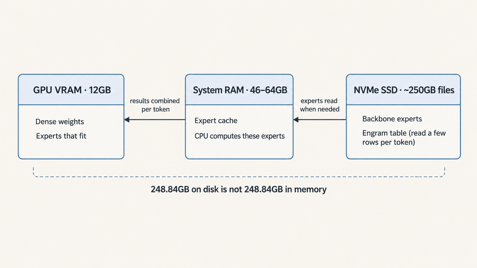
Last verified: 8 November 2026. Both papers are unreviewed working papers, and no outside group has reproduced the results yet. No, AI did not break …
Model Distillation

Model Distillation Explained: When AI Learning Becomes Extraction

Last verified: 7 November 2026. Government and company claims are attributed throughout. None has been tested in court. A support team trains a small, cheap …

Is Claude Faster Than ChatGPT? What the 2026 Benchmarks Show

Claude vs ChatGPT

Benchmarks read from Artificial Analysis on 27 October 2026. UniverseBlend did not run its own timing tests for this article.

Ask a hard question of Claude Opus 5.5 at its maximum effort setting through Anthropic’s API, and the first word of the answer can take more than eleven minutes to arrive. Artificial Analysis recorded a median of 688 seconds on its standard 10,000-token workload. Once the answer starts, it streams at about 96 tokens per second, faster than most of the field. The model is quick to write and very slow to begin.

That gap is the whole story of Claude vs ChatGPT speed. In independent API tests, Claude’s models usually generate text faster than OpenAI’s at comparable settings. At matched effort, Claude Sonnet 5.5 also starts answering sooner than OpenAI’s GPT-6.1 Sol, by 1.2 seconds against 2.9 at the lowest setting. But change the effort level, or compare the budget models, and the faster starter switches sides.

So is Claude faster than ChatGPT? At matched mid-tier settings, yes, by a clear margin. In general, the honest answer is that the reasoning setting you pick moves response time far more than the brand does.

Key Takeaways
  • Time to first token, not tokens per second, dominates total response time for any reasoning-heavy request: at high effort and above, over 70% of a 500-token response is spent waiting.
  • At matched effort, Claude Sonnet 5.5 beat GPT-6.1 Sol on both start time and generation speed at all five levels Artificial Analysis tests.
  • The budget tiers flip it: GPT-6 Luna (Low) starts in 2.1 s against Claude Haiku 5.5 (Low) at 6.7 s, and finishes first on any answer under about 1,360 tokens.
  • The same model can start in about 1 second or about 11 minutes depending on effort, so check the setting before blaming the model.
  • Benchmark medians shift by 10–15% between page loads on the same day. Measure your own prompts before choosing.

Quick Navigation


Claude vs ChatGPT speed: what are we actually measuring?

Claude vs ChatGPT

“Speed” bundles at least six different measurements. Comparisons that quote one and imply another are where most of the confusion comes from.

MetricWhat it measuresHow Artificial Analysis defines it
Time to first token (TTFT)Wait from sending a request to receiving the first tokenIncludes network latency; for reasoning models, the first reasoning token if one is streamed
Time to first answer tokenWait until the first token of the actual answerMeasured after any thinking time
Output speedTokens per second once generation has startedAverage after the first token arrives
End-to-end response timeRequest to complete answerInput processing + thinking + time to produce 500 answer tokens
Reasoning latencyTime spent thinking before or between visible outputNot reported separately; folded into the two figures above
Perceived responsivenessWhen the interface first shows something usefulNot measured; depends on the app

Definitions from the Artificial Analysis performance methodology. It reports the median of the past 72 hours, measured about every three hours from a server in Google Cloud’s us-central1 region, with a 10,000-token prompt as the default workload.

There’s a detail that changes how to read every figure in this article. For Claude Opus 5.5, Sonnet 5.5, GPT-6.1 Sol and GPT-6 Luna, Artificial Analysis lists identical values for time to first token and time to first answer token. Neither provider streams raw reasoning to the client by default. Anthropic’s docs say Claude 5.5 models default to display: "omitted", which skips streaming thinking tokens entirely. OpenAI’s say reasoning tokens are “not visible via the API”. So for these models, “time to first token” really means “time spent thinking, plus a little”.

A simple latency formula

For a streamed response, total time is approximately:

Ttotal≈Tfirst+NremainingRT_{total} \approx T_{first} + \frac{N_{remaining}}{R}

Here T_first is the wait for the first visible token, N_remaining the number of answer tokens still to come, and R the output speed in tokens per second. This is exactly how Artificial Analysis derives its end-to-end figure: Sonnet 5.5 (Low) at 1.17 s plus 500 tokens at 108.9 tokens per second gives the 5.76 s it reports.

The formula ignores tool calls, retries, queueing spikes and the uneven, chunky streaming Anthropic warns about when thinking is on. It still explains most of what users notice, because one of its two terms usually dwarfs the other.

Claude vs ChatGPT speed: what the latest benchmarks show

The fairest comparison available pairs Claude Sonnet 5.5 with GPT-6.1 Sol. They launched within a week of each other in September 2026, cost the same per token ($2 input, $10 output), and Artificial Analysis tests both at the same five effort levels on each provider’s own API.

EffortSonnet 5.5 TTFTGPT-6.1 Sol TTFTSonnet 5.5 output speedGPT-6.1 Sol output speedSonnet 5.5 end-to-endGPT-6.1 Sol end-to-end
Low1.17 s2.86 s109 tok/s43 tok/s5.8 s14.5 s
Medium1.80 s4.90 s108 tok/s45 tok/s6.4 s16.0 s
High12.15 s69.02 s109 tok/s58 tok/s16.8 s77.6 s
Xhigh31.59 s163.06 s112 tok/s53 tok/s36.1 s172.6 s

Source: Artificial Analysis comparison pages for Low, Medium, High and Xhigh, read 27 October 2026. Medians of the past 72 hours; 10,000-token input; first-party APIs. Sonnet variants run with Anthropic’s default fallback enabled.

On this pairing, Claude wins every row: it starts 2.4 to 5.7 times sooner and generates 1.9 to 2.5 times faster. That’s a clean result, but not a complete one. Sonnet 5.5 also writes more. On the same benchmark tasks it produced 14,000 output tokens per task at Low against GPT-6.1 Sol’s 4,000. Faster tokens partly pay for more of them. Artificial Analysis’s estimate of generation time per task (output tokens, thinking included, divided by output speed) puts the two close together: 82 s for Sonnet 5.5 against 93 s for GPT-6.1 Sol at Low.

Other pairings tell different stories:

Pairing (same page)Claude TTFTOpenAI TTFTClaude speedOpenAI speed
Opus 5.5 (Max) vs GPT-6.1 Sol (Max)688.0 s242.2 s96 tok/s62 tok/s
Opus 5.5 (Low) vs GPT-6.1 Sol (Low)8.97 s2.67 s81 tok/s51 tok/s
Haiku 5.5 (Low) vs GPT-6 Luna (Low)6.68 s2.14 s176 tok/s111 tok/s
Sonnet 5.5 (Max) vs GPT-6 Luna (Max)461.9 s93.8 s141 tok/s127 tok/s

Sources: Artificial Analysis comparisons for Opus vs Sol Max, Opus vs Sol Low, Haiku vs Luna Low and Sonnet vs Luna Max, read 27 October 2026.

Across every pairing in these tables, Claude generates faster. Which model starts sooner depends on the pairing. Notice too that GPT-6.1 Sol (Low) read 2.67 s and 51 tokens per second on one page and 2.86 s and 43 tokens per second on another the same day. These are rolling medians, and a 10% gap between two models in a single snapshot is not a result. Public leaderboards have other blind spots too, which we covered in why benchmark scores fail to predict production.

Claude vs ChatGPT speed: why reasoning settings change the result

Every current flagship from both companies reasons before it answers, and both let you set how hard. Anthropic’s Claude API offers five effort levels, Low through Max. Opus 5.5 and Haiku 5.5 default to Medium, Sonnet 5.5 to High. OpenAI’s reasoning effort runs from none to max; GPT-6.1 Sol doesn’t support none or minimal and defaults to Medium.

The effect on waiting time is enormous, and it dwarfs the gap between brands:

Claude Opus 5.5LowMediumHighMax
Time to first token8.97 s10.44 s21.55 s688.0 s
Output speed81 tok/s84 tok/s81 tok/s96 tok/s

Read from Artificial Analysis on 27 October 2026 (Opus Medium vs High, GPT-6 Sol Low vs Max).

Opus 5.5 waits 77 times longer at Max than at Low, while its output speed barely moves. OpenAI’s GPT-6 Sol, the model behind ChatGPT’s Instant mode, shows the same shape: 1.59 s to first token at Low, 132.5 s at Max. That’s the central argument in one row: effort changes how long a model thinks, not how fast it types.

Two cautions keep this honest. First, Anthropic’s thinking is adaptive: at Medium and below, Claude may skip thinking on a simple question, so a quick factual query can start much faster than a 10,000-token benchmark prompt suggests. OpenAI likewise says lower effort favours speed. Second, the two companies’ effort scales are separate designs. “High” on one isn’t calibrated to “High” on the other, so matched-effort tables compare labels, not identical amounts of thought. Capability differs by level too: GPT-6.1 Sol scores higher on Artificial Analysis’s Intelligence Index than Sonnet 5.5 at Low and Medium (42 against 36, 48 against 41), while Sonnet 5.5 leads at Xhigh (52 against 51).

Both providers also sell a paid speed boost. Anthropic’s fast mode promises up to 2.5 times higher output speed on Opus 5.5 at double the price, and says explicitly that it doesn’t shorten time to first token. OpenAI’s fast mode, formerly priority processing, claims up to 2.5 times faster speeds on supported models. Neither fixes the thinking wait.

A fair Claude vs ChatGPT speed test

UniverseBlend didn’t run its own timing tests for this article, so there’s no results table here. What follows is the protocol we’d use, and that you can run.

  1. Pick matched pairs by job, not by brand. Sonnet 5.5 against GPT-6.1 Sol is the closest current pairing on price and release date. Name the effort level for both, and don’t rely on defaults, which differ.
  2. Fix the prompts. Use 20 to 50 real prompts from your workload, identical across models, with the same requested output length.
  3. Stream everything. Record send time, first answer token and last token on the client, using a monotonic clock.
  4. Record the provider’s token counts, not a local tokenizer’s. Claude and OpenAI tokenize differently, so tokens per second aren’t directly comparable across providers. Characters or words per second are a useful cross-check.
  5. Repeat and spread across the day. At least five runs per prompt per model, at different hours. Report the median and the 90th percentile.
  6. Same machine, same region, warm connections. Run both from one client in one cloud region and reuse HTTP connections.
  7. Log failures. Rate limits, 529 overload errors, retries and timeouts are part of speed. Don’t silently drop them.
  8. Keep prompts unique per run, or account for caching. Repeated prefixes can be cached, which cuts processing time and cost.

The main limitation of the public data is the workload: Artificial Analysis uses generated prompts of about 10,000 tokens, which provoke more thinking than a short chat message does. Its numbers are a fair way to compare models on that workload. They won’t tell you your own app’s latency.

Why the fastest model may not feel the fastest

The formula has a consequence that surprises people: a model that starts sooner can lose to a faster generator once the answer gets long enough, and the reverse.

Take the budget tiers. GPT-6 Luna (Low) starts in 2.14 s and generates 111 tokens per second. Claude Haiku 5.5 (Low) starts in 6.68 s but generates 176. Solve for where their total times meet and you get about 1,360 tokens. Below that length, Luna finishes first; above it, Haiku does. A one-paragraph answer favours Luna by several seconds. A long report favours Haiku.

A closer case: Sonnet 5.5 (Low) at 1.17 s and 109 tokens per second against GPT-6 Sol (Low) at 1.59 s and 119 tokens per second. Sonnet shows its first word 0.4 s sooner, and GPT-6 Sol overtakes it after about 540 tokens. Neither difference is one a person would notice. That’s the point: on short interactive turns at low effort, both companies’ fast models start within two seconds, and the choice should be made on quality.

How it feels depends on the job:

  • Everyday questions. Answers are short, so time to first token is nearly the whole experience. Two seconds feels instant; twenty does not.
  • Summarisation. A long document means heavy input processing before anything appears. Generation speed matters less than how quickly the model gets through the input.
  • Coding. People read code as it streams, so a fast start with steady output feels quick even if the full file takes a minute. A model that thinks for two minutes and then dumps the file feels slow even if total time is similar.
  • Research. Users expect to wait. Perceived speed comes from progress signals, not tokens per second.

The apps add their own layer. OpenAI’s ChatGPT help centre says that with its “Intelligent UI” a response may begin while ChatGPT is still thinking. Anthropic’s Claude help centre says thinking can’t be turned off on its 5.5 models, and that higher effort means longer response times. Neither company publishes app latency figures, so app speed can’t be compared from public data.

Claude vs ChatGPT speed: which is better for your workload?

Claude vs ChatGPT

No workload has a universal winner. The table shows which metric to watch and what the current public data does and doesn’t support.

WorkloadMetric that matters mostWhat public data shows (27 Oct 2026)
Short questionsTime to first token at low or medium effortSonnet 5.5 starts 2.4 to 2.7x sooner than GPT-6.1 Sol at Low and Medium; GPT-6 Sol (Low) starts in 1.6 s, close to Sonnet
Long-form writingOutput speedClaude was faster in every matched pairing read; GPT-6 Sol (Low) slightly outpaced Sonnet 5.5 (Low)
Coding and debuggingTotal time per task, plus correctnessNo coding-specific latency data; on Artificial Analysis’s mixed task set at High, estimated generation time per task is 215 s for Sonnet 5.5 against 229 s for GPT-6.1 Sol, close because Sonnet writes more
Deep researchEnd-to-end time including tool callsNo comparable public data; tool latency dominates
Long-context analysisTime to first token at 100k+ inputNot covered by the figures read here; measure it
Agentic workflowsPer-call TTFT multiplied by number of callsNo public end-to-end agent latency comparison
Low-latency API apps90th-percentile TTFT at low effortBudget tier: GPT-6 Luna (Low) 2.1 s against Haiku 5.5 (Low) 6.7 s
High-throughput appsOutput speed under concurrencyHaiku 5.5 (Low) 176 tok/s single-stream; concurrent results not read

Agent workloads deserve a note. An agent that makes ten sequential model calls pays the time-to-first-token cost ten times, so a model that thinks for 12 seconds per call adds two minutes before any tool even runs. Our explainer on how AI agents work and what they cost shows how quickly call counts multiply. For agents, effort per call is usually a bigger lever than model choice.

How to measure AI response speed yourself

The public numbers describe one workload from one data centre. Yours will differ, and measuring it takes an afternoon. These two functions time a streamed response on each provider’s official Python SDK and return time to first answer token, total time, and visible output tokens.

import time
import anthropic
from openai import OpenAI

claude = anthropic.Anthropic()
oai = OpenAI()

def time_claude(prompt, model="claude-sonnet-5-5", effort="medium"):
    t0 = time.perf_counter()
    first = None
    with claude.messages.stream(
        model=model,
        max_tokens=8000,
        output_config={"effort": effort},
        messages=[{"role": "user", "content": prompt}],
    ) as stream:
        for event in stream:
            if (first is None and event.type == "content_block_delta"
                    and event.delta.type == "text_delta"):
                first = time.perf_counter()
        msg = stream.get_final_message()
    end = time.perf_counter()
    u = msg.usage
    thinking = getattr(getattr(u, "output_tokens_details", None), "thinking_tokens", 0) or 0
    return first - t0, end - t0, u.output_tokens - thinking

def time_openai(prompt, model="gpt-6.1-sol", effort="medium"):
    t0 = time.perf_counter()
    first, usage = None, None
    stream = oai.responses.create(
        model=model,
        input=prompt,
        reasoning={"effort": effort},
        stream=True,
    )
    for event in stream:
        if first is None and event.type == "response.output_text.delta":
            first = time.perf_counter()
        elif event.type == "response.completed":
            usage = event.response.usage
    end = time.perf_counter()
    reasoning = usage.output_tokens_details.reasoning_tokens
    return first - t0, end - t0, usage.output_tokens - reasoning

Generation speed is then visible tokens ÷ (total time − time to first token). A few caveats before trusting the numbers:

  • Billing counts include thinking. Both providers count reasoning tokens in output_tokens, so subtract them, as above, or you’ll inflate tokens per second.
  • Tokens differ across providers. Each uses its own tokenizer, so also compare characters per second.
  • Defaults differ. Set effort explicitly. Sonnet 5.5 defaults to High on the API and GPT-6.1 Sol to Medium.
  • First text isn’t always first output. A tool call or empty response leaves first unset; handle that case.
  • Variance is the point. Run each prompt at least five times across the day and report the median and 90th percentile. Queueing near capacity hits tail latency first, as our piece on accelerator utilisation explains.

Conclusion

Is Claude faster than ChatGPT? On the closest like-for-like API pairing, Claude Sonnet 5.5 against GPT-6.1 Sol at the same effort, yes: it started answering 2.4 to 5.7 times sooner and streamed roughly twice as fast in Artificial Analysis’s tests. Across every pairing read here, Claude’s models also generated tokens faster.

That isn’t the same as “Claude responds faster”. At maximum effort, Opus 5.5 kept users waiting 688 s against GPT-6.1 Sol’s 242 s. In the budget tier, GPT-6 Luna started three times sooner than Haiku 5.5. And the consumer apps add routing, interface and default settings that no public benchmark measures.

What the evidence supports, firmly, is the order of importance: effort setting first, model tier second, brand a distant third. Before you choose, time your own prompts at the effort level you’d actually ship, and watch time to first token before tokens per second.

Frequently asked questions

Is Claude faster than ChatGPT in 2026?

On matched API settings, usually yes. Claude Sonnet 5.5 started answering sooner and generated faster than GPT-6.1 Sol at every effort level in Artificial Analysis’s October 2026 data. At maximum effort, and between the budget models, OpenAI’s models started sooner. App speed isn’t publicly benchmarked.

Why does Claude sometimes take longer to start answering?

Because it’s thinking first. Claude’s 5.5 models reason adaptively, and their API hides that thinking by default, so nothing appears until the answer begins. Higher effort means more thinking: Opus 5.5 took about 9 seconds to start at Low and 688 seconds at Max on the benchmark workload.

What is time to first token?

It’s the time between sending a request and receiving the first token of the response, including network delay. When a model hides its reasoning, as both Claude and OpenAI’s models do by default, it effectively measures thinking time plus a small overhead.

Is a higher tokens-per-second score always better?

No. Tokens per second only describes speed after output starts. For short answers, the wait before the first token matters more. Haiku 5.5 (Low) generates far faster than GPT-6 Luna (Low), yet Luna finishes first on any answer under about 1,360 tokens.

Does extended thinking make Claude or ChatGPT slower?

Yes, for both. Thinking time is added before the answer appears. GPT-6 Sol’s time to first token rose from 1.6 seconds at Low effort to 133 seconds at Max. Both companies say lower effort favours speed and suits chat and latency-sensitive work.

Which is faster for coding: Claude or ChatGPT?

There’s no public coding-specific latency comparison. On Artificial Analysis’s mixed task set at High effort, which includes coding, estimated generation time per task is close: 215 seconds for Sonnet 5.5 against 229 for GPT-6.1 Sol, because Sonnet generates faster but writes more. Measure your own repository’s tasks, and judge correctness alongside time.

How can I measure Claude and ChatGPT response times myself?

Stream responses through each official SDK and record when you send the request, when the first answer text arrives and when the stream ends. Use identical prompts, set effort explicitly, repeat each test at least five times, and subtract reasoning tokens before calculating tokens per second.

Does API latency differ from the speed of the ChatGPT or Claude apps?

Yes. Apps choose models and default settings for you, may route between modes, and add interface features such as showing a response while the model is still thinking. Neither company publishes app latency figures, so API benchmarks are a guide to the models, not the apps.


Keep reading

Anthropic IPO valuation

Anthropic IPO: The $895 Billion Question Behind Its Valuation

Last updated: 9 November 2026. Latest confirmed development: Anthropic’s amended S-1, filed on 2 November, still leaves the share count and the IPO price range …
Claude Opus vs Sonnet

Claude Opus vs Sonnet: What the 2026 Price Gap Actually Buys

Last verified: 8 November 2026. All prices are Anthropic’s standard first-party API rates in US dollars per million tokens. They aren’t Claude Pro or Max …
RSA-1024

Did AI Break RSA? What DeepMind Actually Found
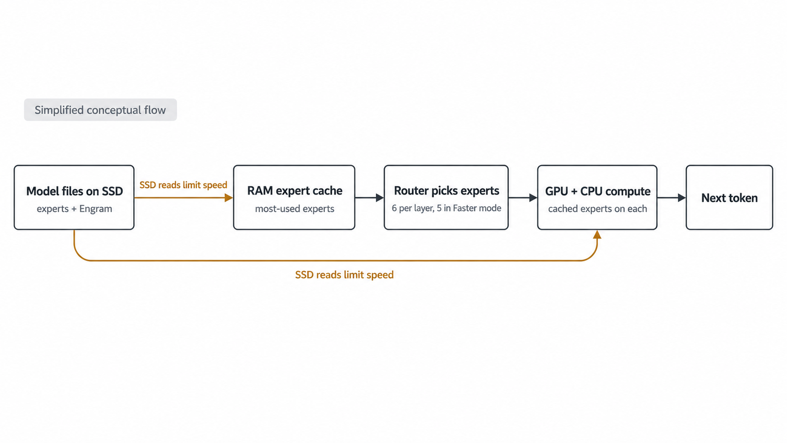
Last verified: 8 November 2026. Both papers are unreviewed working papers, and no outside group has reproduced the results yet. No, AI did not break …
Model Distillation

Model Distillation Explained: When AI Learning Becomes Extraction

Last verified: 7 November 2026. Government and company claims are attributed throughout. None has been tested in court. A support team trains a small, cheap …

Kimi K3.1 Pro Hardware Requirements: GPUs, Memory, Cost

Kimi K3.1 Pro hardware requirements

Last updated: 5 November 2026. Kimi K3.1 Pro’s official weights are now on Hugging Face, so we’ve confirmed the parameter count, expert layout, MXFP4 format and checkpoint size, replaced the K3 licence terms with the published K3.1 Pro licence, corrected the attention layout and added a section on downloading the weights safely.

Before anyone argues about which GPU to rent, a smaller question settles most of the argument: how many bytes have to sit in accelerator memory before the first token comes out? For Kimi K3.1 Pro hardware requirements, that number already exists, even though the model’s own weights don’t.

Moonshot AI launched Kimi K3.1 Pro on its API on 23 October and describes it as a post-trained version of Kimi K3. K3’s weights have been public since July, and they occupy 1.561 TB. Unless Moonshot changes the format when it publishes K3.1 Pro, that’s the floor: about 1.56 TB of weights before a single cached token, activation buffer or draft model.

A model name doesn’t give you a GPU count. Weight format, memory per accelerator, the engine’s reservation, context length and concurrency do. This guide works through each with the arithmetic shown, so you can swap in your own numbers.

Quick Answer
  • Weights released: Kimi K3.1 Pro’s official weights went live on Hugging Face at the start of November 2026, under the moonshotai organisation.
  • Model size: 2.8T total parameters with 104B active, shipped as a 1.56 TB MXFP4 checkpoint split across 96 files.
  • Memory needed: about 1.6 TB of GPU memory for the weights alone, before KV cache.
  • Minimum GPUs: eight 288 GB GPUs (B300, GB300 or MI355X) as a floor, 16 B200 or H200 cards, or 24 to 32 H100s. These are our estimates, since Moonshot publishes no minimum hardware.
  • Long context: the 1M-token window adds up to about 18 GB per request on our revised estimate.
  • Licence: the Kimi K3.1-Pro License is MIT-style, with extra conditions above $20M in revenue or 100M monthly users.
  • Download safely: use only the official moonshotai repository and verify the files before you load them.
Key Takeaways
  • The official weights are out: 2.8T total parameters, 104B active, 1.56 TB across 96 safetensors shards on Hugging Face.
  • Fake and repackaged Kimi K3.1 Pro uploads are likely to follow, so download only from the moonshotai organisation and verify model weights before you download.
  • “2.8 TB at 8-bit” is arithmetic for a file that doesn’t exist. The native release is already 4-bit, trained that way.
  • Eight 288 GB GPUs in one node are the floor. B200, H200 and H100 fleets need two or more nodes just to hold the weights.
  • Every request costs a fixed 0.2 to 0.4 GB of KDA state plus about 14 KB per token of FP8 MLA cache, so short requests aren’t as cheap as their length suggests and million-token contexts are cheaper than on dense models.
  • A single on-demand AWS node costs about $102,540 a month before redundancy, staff or storage.
  • Matching the $2/$10 API on a 20k-in, 2k-out workload takes roughly 13,000 input and 1,300 output tokens per second, sustained around the clock. Measure whether your hardware can do that before you sign anything.
  • The K3 licence isn’t MIT: model-as-a-service businesses above $20 million in total company revenue need a separate agreement.

Quick Navigation


What is confirmed about Kimi K3.1 Pro

With the weights released on Hugging Face, every core specification on this page now comes from Moonshot’s own model card and config.json rather than from Kimi K3.

SpecificationKimi K3.1 ProSource
Total parameters2.8TModel card
Active parameters per token104BModel card
Layers93 (1 dense)Model card
Attention layout69 KDA (linear attention) + 24 Gated DSA (sparse attention)Model card, config.json
Experts896, with 16 routed + 2 shared per tokenconfig.json
Hidden size / attention heads7168 / 96Model card
Weight formatMXFP4 weights, MXFP8 activations, quantization-aware trainingModel card
Context window1,048,576 tokensconfig.json
Vision encoderMoonViT-V2, 401M parametersModel card
Checkpoint size1.56 TB, 96 safetensors shardsHugging Face file tree
Recommended enginesvLLM, SGLang, TokenSpeedModel card
APILive as kimi-k3.1-proKimi blog

One change from Kimi K3 matters for memory planning. K3.1 Pro swaps K3’s 24 full-attention Gated MLA layers for Gated DSA, a sparse attention design, which changes the KV cache figures below. Moonshot doesn’t state minimum hardware anywhere in the release, so the GPU counts on this page remain our estimates from the published sizes.

Calculating Kimi K3.1 Pro weight memory

Kimi K3.1 Pro hardware requirements

The formula is plain: weight bytes = parameters x bits per parameter ÷ 8. Using K3’s 2,779,931,837,184 parameters:

PrecisionBits per parameterDecimal TBBinary TiBWhat it represents
BF16165.5605.057Theoretical; no such release
8-bit (FP8/INT8)82.7802.528Theoretical
4-bit, no scales41.3901.264Theoretical minimum
MXFP4 everywhere4.251.4771.343Adds one 8-bit scale per 32 weights
Actual K3 checkpoint4.49 (effective)1.5611.420Published repository, 96 shards

The released checkpoint confirms the MXFP4 estimate. Moonshot’s config lists the format as mxfp4-pack-quantized with one scale per group of 32 weights, and the Hugging Face repository totals 1.56 TB across 96 shards. Plan for about 1.6 TB of memory for weights, plus room for the vision encoder, KV cache and runtime overhead.

All rows are weights only, with no runtime overhead. The brief’s “2.8 TB at 8-bit, 1.4 TB at 4-bit” is correct arithmetic for the wrong question. Moonshot trained K3 to run in MXFP4 from supervised fine-tuning onward, so there is no 8-bit release to plan around.

The gap between 1.39 TB and 1.561 TB has two sources. MXFP4 stores a shared 8-bit scale for every block of 32 weights, adding about 0.09 TB. And the config leaves attention, shared experts, the dense first-layer MLP, the output head and the vision encoder unquantized. The “5.6 TB” figures circulating for K3 come from assuming BF16.

Watch your units. TB is 10^12 bytes and TiB is 2^40, about 10% larger. NVIDIA lists a DGX B300’s total GPU memory as “2.1 TB”, yet eight 288 GB GPUs hold 2,304 GB, which is 2.10 TiB. Compare a TiB capacity with a TB weight file and you’ve lost a tenth of your headroom on paper.

How many GPUs Kimi K3.1 Pro needs

The lower bound is: GPUs = ceiling(weight bytes ÷ (memory per GPU x usable fraction)). vLLM’s Kimi K3 recipes run at 0.88 to 0.92 of GPU memory; this guide uses 0.90.

AcceleratorMemory per GPULower boundPractical layoutFits one 8-GPU node?
NVIDIA B300 / GB300288 GB78Yes, ~513 GB left after weights
AMD MI355X288 GB78Yes, same arithmetic
NVIDIA B200180 GB1016 (two nodes)No: 1,440 GB total
NVIDIA H200141 GB1316 (two nodes)No: 1,128 GB total
NVIDIA H10080 GB2224 to 32 (three to four nodes)No

Memory per GPU from AMD’s MI355X page (which also lists B200 at 180 GB) and NVIDIA. Seven 288 GB GPUs clear the bound, but tensor parallelism splits the 96 attention heads across GPUs, and 96 doesn’t divide by seven. Eight is the real floor, and it’s what the vLLM recipe states: at least 8x GB300, or 8x MI355X/MI350X on ROCm, with “multi-node for real production traffic”.

Eight GPUs are not one 2.3 TB pool. Each holds its own shard, and every layer exchanges activations between them. Inside a DGX B300 that traffic rides NVLink at 14.4 TB/s aggregate. Between nodes it crosses InfiniBand or Ethernet at up to 800 Gb/s per port, roughly 100 GB/s, which is why two-node recipes split the model into pipeline stages (TP8 x PP2) and why NVIDIA’s Dynamo recipes target GB200 and GB300 racks with NVLink spanning trays: 16 GB200s aggregated, or 32 split between prefill and decode.

Hopper is the awkward case. H100 and H200 lack native FP4 tensor cores, so MXFP4 experts run through dequantising kernels. The recipe page builds commands for H200, but its stated minimum is Blackwell or MI355X, and we found no published throughput for K3 on Hopper.

Can a single GPU or workstation run it?

No single GPU comes close. The workstation route is llama.cpp with the experts in system RAM. One published test loaded a ~554 GB 1-bit GGUF of K3 on a 160 GB VRAM machine with the MoE weights on CPU. Nobody has published quality figures for that quant. The 4-bit GGUF is 1,508.7 GB, barely smaller than the native file, because the native file is already 4-bit. It’s a way to poke at the model, not to serve users, and Now that the weights are public, community quants of Kimi K3.1 Pro can appear, but none are official, and their quality and memory use are unverified until someone tests them. The K3 result above (a 554 GB 1-bit GGUF reportedly running on 160 GB of VRAM) is the best guide for now. Before you run any community build, put it through the checks in our model weights verification guide..

The KV cache changes the Kimi K3.1 Pro calculation

This is the one part of the page where the release changed our numbers. Our first estimate assumed K3’s Gated MLA layers. Kimi K3.1 Pro uses Gated DSA in those 24 layers instead, and its config gives the inputs for a revised estimate.

  • DSA layers: the config keeps a 512-value compressed KV latent plus a 64-value positional key (576 values), and adds a lightning indexer with a 128-dimension key. Assuming each of the 24 layers caches both, as DeepSeek’s DSA does, that’s 24 × (576 + 128) = 16,896 values per token, or about 16.9 KB at FP8.
  • KDA layers: these keep a fixed-size state rather than a growing cache. At 69 layers × 96 heads × 128 × 128 values in BF16, that’s about 0.22 GB per request, whatever the context length.
Context lengthDSA cache (FP8)KDA stateTotal per request (estimate)
8K tokens0.14 GB0.22 GB0.36 GB
32K tokens0.55 GB0.22 GB0.77 GB
128K tokens2.21 GB0.22 GB2.43 GB
256K tokens4.43 GB0.22 GB4.65 GB
1M tokens17.72 GB0.22 GB17.93 GB

Treat these as planning estimates, not measured figures. Moonshot hasn’t published KV cache sizes, and vLLM or SGLang may store the cache differently. The indexer only picks the top 2,048 earlier tokens for each query (index_topk in the config), which saves compute, but the full cache still has to sit in memory. Check your engine’s own memory report once the model loads.

Two things fall out. Below about 16,000 tokens the fixed state outweighs the growing cache, so short chat traffic carries a per-request floor most sizing guides ignore. At the other end, long contexts are cheap: a 70B dense model with grouped-query attention needs about 160 KB per token, as our breakdown of AI memory costs works out, or roughly 172 GB for a million tokens against K3’s 14.7 GB.

On one 8x B300 node, 0.90 of 2,304 GB leaves about 2,074 GB, and weights take 1,561 GB. Set aside an assumed 110 GB for activations, CUDA graphs, communication buffers and the speculative draft model the recipes load, and roughly 400 GB remains for requests. That’s an upper bound of about 600 concurrent requests at 32K, 197 at 128K, or 27 at the full million.

Those counts assume the cache is spread across GPUs without duplication. vLLM’s decode context parallelism does that for MLA; without it, tensor-parallel ranks can each hold a copy and the numbers fall sharply. The recipes also spill to host RAM: one AMD prefill configuration budgets 1,799 GB of host DRAM for cache offload. Memory scales linearly with concurrency and context. Throughput at those concurrencies is a separate question that only measurement answers.

Where to download Kimi K3.1 Pro weights safely

The only official source is the moonshotai/Kimi-K3.1-Pro repository on Hugging Face. A 1.56 TB download is a big target for copycats, and a fake or tampered upload costs you days of transfer time and GPU hours before you notice anything is wrong.

There’s a second reason to be careful with this release. The repository ships its own Python files, and Moonshot’s usage example loads them with trust_remote_code=True. A mirror that changes those files can run code on your servers the moment you load the model. Our guide to spotting fake model weights walks through seven checks before you download. For Kimi K3.1 Pro, the short version is:

  1. Check the organisation. The repo should sit under moonshotai, the same Hugging Face account that hosts Moonshot’s earlier Kimi K3 release.
  2. Check the file list. Expect 96 safetensors shards totalling about 1.56 TB, plus config.json, the LICENSE and the custom code files. Pickle or .bin weight files are a warning sign.
  3. Read the custom code before you trust it. If you pull from anywhere other than the official repo, compare the .py files against Moonshot’s versions line by line.
  4. Compare hashes. Hugging Face shows a SHA-256 for each large file. Match your local copies against the official repo, not against the mirror you downloaded from.
  5. Treat quants as third-party software. Moonshot hasn’t released any official quantised variants. Any GGUF or lower-bit build is a community conversion, so check who made it and what it was built from.

Quantisation trade-offs

Weight quantisation and cache quantisation are separate levers, and the first one is mostly pulled already.

LeverMemory effectWhat you risk
Keep native MXFP4 weightsBaseline 1.561 TBNothing; this is how the model was trained
Up-cast to FP8 or BF161.8x to 3.6x moreHardware cost, with no documented quality gain
Community 1-bit or 2-bit quantsAbout 0.55 TB for the smallest published 1-bit GGUFUnmeasured quality loss; K3-only until K3.1 Pro weights ship
FP8 KV cacheHalves the MLA cache versus BF16Small accuracy risk; recipes use it by default
FP32 vs BF16 KDA stateDoubles or halves the fixed per-request stateSome low-latency backends require FP32

Because K3 went through quantization-aware training, its 4-bit weights aren’t a lossy copy of some better original that’s available to you. Going below 4 bits is a real compression, and nobody has published K3 or K3.1 Pro quality numbers for those quants. Run your own evaluation against the hosted API before trusting one.

Hardware matters here too. Blackwell and AMD’s CDNA 4 parts execute MXFP4 natively; AMD lists 10.1 PFLOPs of MXFP4 matrix throughput for the MI355X. Hopper doesn’t, which is a second reason the recipes start at Blackwell. The cache side has its own knobs: the latency-tuned GB300 profile switches the KDA state to FP32, doubling that per-request floor to about 0.43 GB.

The real cost of self-hosting Kimi K3.1 Pro

Kimi K3.1 Pro hardware requirements

Two dated price points for one 8x B300 node, on demand, 30 days at 24 hours:

ItemAWS p6-b300.48xlargeMedian specialist cloud
Hourly, 8x B300$142.42$65.44 ($8.18 per GPU)
30 days continuous (720 h)$102,540$47,117
Effective rate at 50% useful utilisation$284.83/h$130.88/h
Effective rate at 25% useful utilisation$569.66/h$261.76/h

AWS rate: us-east-1, Linux, on demand, per Vantage’s EC2 tracker, read 26 October 2026; the instance includes 4,096 GiB of host RAM and 8 x 3.84 TB local NVMe. Specialist rate: median across 10 providers per getdeploying, 8 September 2026; those offers may not match AWS on networking, storage or availability.

The effective-rate rows are the ones that matter. A node you pay for around the clock but keep busy half the time costs twice as much per useful hour, and real traffic has nights and weekends.

The GPU line also isn’t the bill. One node has no redundancy, so a production service needs a second, doubling the fixed cost before it serves an extra token. Add engineering time, monitoring, storage for 1.56 TB of weights plus staging on every node, egress, and the work of swapping in K3.1 Pro weights when they arrive. Published estimates of that total put it at 1.3 to 5 times the raw GPU rate, a range we unpack in the hidden fees in self-hosted LLM cost.

Kimi K3.1 Pro API vs self-hosting: the break-even

Moonshot’s API price for standard kimi-k3.1-pro is $2 per million input tokens, $10 per million output and $0.20 per million cached input, confirmed by Artificial Analysis. The Highspeed variant costs $4/$20. Cache writes are billed separately at a rate that wasn’t displayed when we checked.

The formula: API cost = (input tokens ÷ 1,000,000 x input rate) + (output tokens ÷ 1,000,000 x output rate).

Illustrative workload, an assumption: an agentic coding call with 20,000 input tokens and 2,000 output tokens, reasoning included. Uncached, that’s $0.04 + $0.02 = $0.06 per call. With 90% of input served from cache, it’s $0.0076 + $0.02 = $0.0276, before cache-write fees.

Break-even calls per month = monthly self-hosting cost ÷ API cost per call. Spread over 2,592,000 seconds in 30 days:

Scenario (GPU cost only)Calls/month to match APISustained calls/sInput tokens/sOutput tokens/s
AWS, no cache1.71M0.6613,1871,319
AWS, 90% cache hits3.72M1.4328,6672,867
Specialist cloud, no cache785K0.306,059606
Specialist cloud, 90% cache hits1.71M0.6613,1721,317

Caching makes the API cheaper, so it pushes break-even further away. And these are averages held for 720 hours straight. Peaks need headroom above them, so a fleet that just breaks even on average is running below capacity most of the day.

Can one node sustain those rates at an acceptable latency? There’s no independent published throughput for K3.1 Pro on 8x B300, so that’s the number to measure, not assume. Remember too that the right comparison is the cheapest API that meets your quality bar. Third-party hosts listed K3 below Moonshot’s own price on OpenRouter, and the same is likely once K3.1 Pro weights circulate. Our Kimi K3.1 Pro vs Sonnet 5.5 comparison covers per-task token use, which moves the API side of this equation more than the rate card does.

Self-hosting earns its place when data can’t leave your infrastructure, when load is high and steady enough to keep a node busy, when you need to fine-tune, or when you already own Blackwell capacity sitting idle.

Licence and operational constraints

Moonshot published the Kimi K3.1-Pro License with the weights. It starts as an MIT-style licence, then adds three conditions that matter for self-hosting.

  • Model-as-a-Service: if you sell access to the model and earn more than $20M in aggregate revenue over any consecutive 12 months, you need a separate agreement with Moonshot.
  • Attribution: a product with more than 100 million monthly active users, or more than $20M in monthly revenue, must prominently display “Kimi K3.1-Pro”.
  • Exemptions: internal use is exempt, as is use through Moonshot’s official products or certified inference partners.

For most teams running the model in-house, the licence won’t change the hardware decision. If you plan to resell inference at scale, email license@moonshot.ai before you buy GPUs. This is a summary, not legal advice, so have your counsel read the full text.

A practical Kimi K3.1 Pro deployment decision

  • Use the hosted API when traffic is small, spiky or unproven, or nobody on the team runs GPU clusters. Moonshot offers zero data retention to API customers, which settles some privacy objections without any hardware.
  • Rent one 8x B300 or MI355X node for evaluations, fine-tuning experiments or steady internal batch work you can keep busy. Accept that it has no redundancy.
  • Plan multi-node or rack-scale for production with latency targets, long contexts at high concurrency, or uptime commitments. Moonshot’s 64-plus accelerator guidance describes this tier.
  • Benchmark before you sign. Replay 50 to 200 real requests, measure tokens per second at your p95 latency target, and compare any quantised variant’s outputs with the hosted API.

What would change this estimate? The K3.1 Pro file size and precision; the KDA state dtype your engine uses; your measured throughput per node; GPU rental prices, which roughly doubled for B300 through 2026 according to price trackers; and the K3.1 Pro licence terms.

Conclusion

Kimi K3.1 Pro’s weights are now public, and they match the estimates this page made before launch: a 1.56 TB MXFP4 checkpoint that needs about 1.6 TB of GPU memory before KV cache. Eight 288 GB GPUs remain the practical floor, and the 1M-token context adds up to about 18 GB per request on our revised estimate. For most teams the API is still the cheaper route unless usage is heavy and steady. If you do self-host, start from the official moonshotai repository and verify the files before anything touches your cluster.

So don’t rent for Kimi K3.1 Pro hardware requirements yet. Use the API, log your real token mix and concurrency, and when the weights land, check the file size against 1.56 TB, then spend a week on one rented node measuring tokens per second at your latency target. If that number can’t clear the break-even rates in the table above with room for peaks and a second replica, the API was the cheaper machine all along.

Frequently asked questions

How much VRAM does Kimi K3.1 Pro need?

About 1.6 TB for the weights alone, based on the official 1.56 TB MXFP4 checkpoint, plus KV cache and overhead. That’s eight 288 GB GPUs at minimum, 16 B200 or H200 cards, or 24 to 32 H100s. Moonshot doesn’t publish minimum hardware, so these counts are our estimates.

Can Kimi K3.1 Pro run on one GPU?

No. The largest current accelerators, NVIDIA B300 and AMD MI355X, hold 288 GB each, under a fifth of the 1.56 TB weight file. Even heavily compressed community quants of K3 run to roughly 550 GB, which still needs several GPUs or large amounts of system RAM.

How many GPUs are needed for a model of this size?

Eight 288 GB GPUs are the practical minimum and match the vLLM recipe’s stated floor. With 180 GB B200s or 141 GB H200s you need 16 across two nodes. Moonshot recommends 64 or more accelerators for efficient production serving.

Does 4-bit quantisation reduce memory requirements?

For this model it’s already applied. Kimi K3 ships in MXFP4, a 4-bit format with shared scales, trained that way from fine-tuning onward. Converting to 8-bit would roughly double memory. Going below 4 bits shrinks the file further, but no published quality data exists for those quants.

How much does self-hosting cost per month?

One 8x B300 node costs about $102,540 for 30 days on AWS on demand, or about $47,117 at the median specialist-cloud rate (prices checked September to October 2026). Redundancy, staff, storage and idle time add substantially to that GPU line.

Is an API cheaper than running the model locally?

For most workloads, yes. At $2/$10 per million tokens, a self-hosted AWS node only matches the API if it sustains about 1.7 million 20k-token calls a month. Self-hosting can win on data control, steady high load or fine-tuning needs.

Can I run Kimi K3.1 Pro on a workstation?

Not at the official precision. The checkpoint is far larger than any workstation’s memory. Community quants may make heavily compressed versions possible, as a 1-bit GGUF did for Kimi K3, but none are official and quality is untested.

What licence applies to commercial deployment?

The Kimi K3.1-Pro License, an MIT-style licence with extra conditions. Model-as-a-Service businesses earning over $20M in 12 months need a separate agreement, and products above 100M monthly users or $20M monthly revenue must display “Kimi K3.1-Pro”. Internal use is exempt.

Where can I download Kimi K3.1 Pro safely?

Only from the official moonshotai/Kimi-K3.1-Pro repository on Hugging Face. Check the organisation, file list and hashes before downloading, and see our guide to verifying model weights for the full checklist.


Keep reading

Anthropic IPO valuation

Anthropic IPO: The $895 Billion Question Behind Its Valuation

Last updated: 9 November 2026. Latest confirmed development: Anthropic’s amended S-1, filed on 2 November, still leaves the share count and the IPO price range …
Claude Opus vs Sonnet

Claude Opus vs Sonnet: What the 2026 Price Gap Actually Buys

Last verified: 8 November 2026. All prices are Anthropic’s standard first-party API rates in US dollars per million tokens. They aren’t Claude Pro or Max …
RSA-1024

Did AI Break RSA? What DeepMind Actually Found
Last verified: 8 November 2026. Both papers are unreviewed working papers, and no outside group has reproduced the results yet. No, AI did not break …
Model Distillation

Model Distillation Explained: When AI Learning Becomes Extraction

Last verified: 7 November 2026. Government and company claims are attributed throughout. None has been tested in court. A support team trains a small, cheap …

Kimi K3.1 Pro vs Sonnet 5.5: Same Price, Different Bill

Kimi K3.1 Pro

On paper, Moonshot AI priced Kimi K3.1 Pro to the cent against Claude Sonnet 5.5: $2 per million input tokens and $10 per million output tokens. Run both through the same independent test suite, though, and the bills part ways. Artificial Analysis spent an average of $2.11 per task running Kimi K3.1 Pro through its Intelligence Index. Sonnet 5.5 at maximum effort cost $5.46 per task on the same evaluations.

The token price is identical. The cost of the work is not, and that gap matters more than any score Moonshot published when it released the model on 23 October 2026.

The second thing to know is that Kimi K3.1 Pro is not yet an open-weight model. Moonshot says the full weights will be released by 4 November. Until they appear, it is a hosted API like Sonnet 5.5, and the questions that come with downloadable weights are still ahead.

This comparison was researched on 26 October 2026. It weighs Kimi K3.1 Pro against Claude Sonnet 5.5 and Claude Opus 5.5 on independently measured capability, list price, measured cost per task, and what changes when weights ship. Provider-reported figures are labelled throughout.

Key Takeaways
  • Kimi K3.1 Pro and Sonnet 5.5 share a $2/$10 list price, but Sonnet 5.5’s cache reads cost $0.10 per million tokens against Kimi’s $0.20.
  • On Artificial Analysis’s Intelligence Index v4.3.2, Kimi K3.1 Pro scores 55, Sonnet 5.5 56 and Opus 5.5 58. A one-point gap does not show either model is better.
  • Terminal-Bench 4.0 rankings flip with the harness: vendor numbers put Sonnet 5.5 first, while Artificial Analysis’s run puts Kimi K3.1 Pro first at 67.2%.
  • Kimi K3.1 Pro used about a quarter of Sonnet 5.5’s output tokens per index task at max effort, which is why it cost $2.11 per task against $5.46.
  • Weights are promised by 4 November 2026. Serving 2.8 trillion parameters is a multi-GPU data-centre job, not a workstation install.

Quick Navigation


The price comparison needs a footnote

The list prices are where the “same price” claim holds.

Per 1M tokensInputOutputCache hitCache write
Kimi K3.1 Pro$2.00$10.00$0.20Billed by TTL; rate not displayed at research date
Claude Sonnet 5.5$2.00$10.00$0.10$2.50 (5 min), $4.00 (1 h)
Claude Opus 5.5$4.00$20.00$0.20$5.00 (5 min), $8.00 (1 h)

Sources: Kimi API docs, Artificial Analysis, Anthropic pricing. Prices checked 26 October 2026.

Input matches input and output matches output; Opus 5.5 is exactly double. Three footnotes complicate the picture.

  1. Cache reads. Anthropic charges 5% of the input rate for Sonnet 5.5 cache hits. Kimi charges 10%. For an agent that re-reads the same long prefix on every call, that difference compounds. Kimi also bills cache writes separately, and the write rate was not displayed on its pricing page when we checked.
  2. Tokenizers. Anthropic says its current tokenizer produces roughly 30% more tokens for the same text than its older one. Kimi uses its own tokenizer, and we found no public comparison of the two. A million tokens on each platform may not hold the same amount of text.
  3. Speed. Artificial Analysis measured Kimi K3.1 Pro at about 58 output tokens per second on Moonshot’s API, against about 134 for Sonnet 5.5. Moonshot’s Highspeed variant runs two to three times faster at double the price, except for cache hits. If latency matters, the comparable Kimi price is closer to $4/$20.

So the headline survives, narrowly: same list price for uncached input and output, and nothing more.

What Kimi K3.1 Pro actually changes

Kimi K3.1 Pro is not a new architecture. Moonshot describes it as Kimi K3, released in July, with substantially more post-training compute spent on reinforcement learning across hundreds of domains. The price fell from K3’s $3/$15.

The model is a mixture-of-experts (MoE) design: a router sends each token through a small subset of specialist sub-networks instead of the whole model. Artificial Analysis lists 2.8 trillion total parameters with about 104 billion active per token. Coverage of the K3 launch reported 896 experts with 16 active per token; Moonshot has not restated that for K3.1 Pro.

Reasoning is always on. The API offers low, high and max effort, defaults to max, and fixes temperature at 1.0. Moonshot’s benchmark claims all use max.

What the 1M-token context window means

Moonshot lists a 1,048,576-token window for the K3 series, shared between input and output, with a default output cap of 131,072 tokens. Sonnet 5.5 and Opus 5.5 also offer 1M tokens at standard pricing.

A window is capacity, not proof of quality. The longest independent test here, AA-LCR v1.1, uses documents of roughly 10,000 to 100,000 tokens. Kimi K3.1 Pro scores 86%, Opus 5.5 85% and Sonnet 5.5 83%. That is encouraging, but it says nothing direct about reasoning across 800,000 tokens.

Why 2.8 trillion parameters is not a normal open-weight deployment

MoE cuts compute per token. It does not cut memory. The router can call any expert, so all 2.8 trillion parameters must sit in accelerator memory even though only about 104 billion fire per token.

K3’s published weights, the closest reference, came to about 1.56 TB on Hugging Face. Vast.ai lists full-precision K3 serving on an eight-GPU B300 node, plus 1-bit and 2-bit community quantizations that fit one node at some cost in accuracy. Long-context key-value caches come on top.

An 8-billion-parameter open model runs on one consumer GPU. A licence page puts both in the “open weights” category. Operationally, Kimi K3.1 Pro belongs in a data centre.

Kimi K3.1 Pro vs Sonnet 5.5: the benchmark evidence

Kimi K3.1 Pro

Independent figures come from Artificial Analysis, which runs every model through the same harness. Provider figures come from Moonshot’s and Anthropic’s launch materials.

MeasureKimi K3.1 ProSonnet 5.5Opus 5.5Source type
AA Intelligence Index v4.3.2555658Independent
Terminal-Bench 4.0, AA harness67.2%63.6%59.6%Independent
Terminal-Bench 4.0, provider65.7%70.6%66.4%Provider-reported
Humanity’s Last Exam52%55%61%Independent
AA-Omniscience (−100 to 100)303246Independent
AutomationBench-AA73%72%70%Independent
AA-Briefcase v1.1 (Elo)1,6781,8161,801Independent

Independent rows test Sonnet 5.5 and Opus 5.5 at “Max, Default Fallback”. Moonshot’s own score used a Claude Code harness. Anthropic’s Opus figure is its xhigh run; at max it reported 64.8%. Sources: AA Kimi vs Sonnet, AA Kimi vs Opus, AA Terminal-Bench 4.0, Moonshot.

What a one- or three-point gap means

Artificial Analysis presents point scores without error bars, so a one-point gap between Kimi K3.1 Pro and Sonnet 5.5 is best read as a tie. A tie on the composite does not make the models equivalent, because the components disagree.

Kimi K3.1 Pro leads on terminal work, SaaS automation and long-context reasoning. It trails on knowledge: 52% on Humanity’s Last Exam against Opus 5.5’s 61%, and 30 on AA-Omniscience against 46. AA-Omniscience penalizes hallucinated answers, so that 16-point gap matters wherever a confident wrong fact is expensive. On AA-Briefcase, which grades long-horizon deliverables such as memos and spreadsheets, both Claude models lead by more than 120 Elo points.

The Terminal-Bench ranking flips with the harness

In vendor reporting, Sonnet 5.5 leads Terminal-Bench 4.0 at 70.6%, Opus 5.5 follows at 66.4% and Kimi K3.1 Pro is third at 65.7%. In Artificial Analysis’s run the order reverses: Kimi 67.2%, Sonnet 63.6%, Opus 59.6%.

These are different experiments, not contradictory ones. Artificial Analysis runs all 66 tasks with the mini-swe-agent harness and averages pass@1 over three repeats. Moonshot ran its model in a Claude Code harness and took rivals’ scores from their blogs or the official leaderboard, whichever was higher.

Scale matters too. With 66 tasks, one task is worth about 1.5 points, so Kimi’s 3.6-point independent lead over Sonnet 5.5 is two or three tasks per pass. What both sets agree on is that the three models are close and the harness moves results by several points, a pattern our LLM benchmark comparison found across other models.

Before transferring any ranking to your workload, ask:

  • Does the harness resemble your agent framework, tools and permissions?
  • Which effort level was tested, and can you afford it in production?
  • How many tasks separate the models, and were scores averaged over repeats?
  • Do failures arrive loudly as errors or quietly as plausible wrong output?
  • What are time to first token and total time per task?

The last question has teeth. At max effort, Artificial Analysis measured Sonnet 5.5’s time to first token at about 372 seconds, against about 3 seconds for Kimi K3.1 Pro; total time per task was closer, at 936 and 846 seconds. We cover why public scores rarely transfer in why benchmark scores fail to predict production.

The token price is not the cost of the job

Kimi K3.1 Pro

A per-token price multiplies by token count, and token counts differ sharply. Artificial Analysis recorded what each model produced across its index:

AA Intelligence Index v4.3.2Kimi K3.1 ProSonnet 5.5 (max)Opus 5.5 (max)
Output tokens per task55k197k119k
of which reasoning35k147k84k
Cost per task$2.11$5.46$5.98
Cost to run full index$3,117$7,260$8,708

At max effort, Sonnet 5.5 reasons for roughly four times as many tokens as Kimi K3.1 Pro. Identical prices times very different volumes produce bills about 2.6 times apart.

Effort is a dial, though. In September, Artificial Analysis reported Sonnet 5.5 at xhigh scoring 52 for $2.74 per task, priced before Anthropic halved its cache-read rate. Lower effort narrows the cost gap and widens the capability gap, so compare models at the effort each would really run at.

Three illustrative workloads

These figures are illustrative arithmetic at list prices, not measurements. They ignore tokenizer differences and batch discounts.

Scenario and assumptionsKimi K3.1 ProSonnet 5.5Opus 5.5
1. Document analysis: 200k input, 4k output, no cache$0.44$0.44$0.88
2. Coding task: 30k input plus each model’s AA-measured average output (55k / 197k / 119k)$0.61$2.03$2.50
3. Cached agent loop: 100k prefix, 50 calls, 2k fresh input and 3k output per call, one cache write then 49 hits$2.68 plus write fee$2.44$4.88

Scenario 1 is the headline claim working as advertised: input-heavy work costs the same on both. Scenario 2 shows where it breaks, because a model that generates more tokens turns the same rate card into a bill three times larger. Scenario 3 reverses direction: Sonnet 5.5’s cheaper cache reads win even before Kimi’s unpublished write fee, which would add about $0.25 if it matched Anthropic’s 5-minute rate (an assumption).

Scenario 3 also holds output constant across models, which scenario 2 shows is unrealistic. Only your own traces can say which effect dominates.

What self-hosting adds

Once weights ship, a per-token bill can become a per-hour bill. Hourly hardware cost ÷ tokens per second ÷ 3,600 × 1,000,000 gives cost per million tokens. The hard part is the inputs: a multi-GPU node, a throughput figure measured at your batch size, and utilization, since an idle accelerator still bills by the hour.

Add engineering time for serving software, quantization testing, monitoring, security patching and updates. Self-hosting is not cheaper by default; it wins only at sustained high utilization, as we showed in what inference actually costs per token.

Kimi K3.1 Pro open weights change the security equation

Moonshot paired the launch with an unusual disclosure. It says it found cyber-related content in its mid-training corpus and cyber tasks in its reinforcement-learning mix, and removed both ahead of the open release while keeping general coding tasks.

Its evidence is xdev-bench-hard, an in-house test in which an agent must turn a known vulnerability in software such as the Linux kernel or Node.js into a working exploit. At pass@3 with no hard timeouts, a checkpoint trained without filtering solved 90.5% of tasks, the released K3.1 Pro 81.0% and Kimi K3 33.3%. On Moonshot’s own test, filtering lowered the ceiling. It also left most of the capability in place, because general coding skill transfers.

The independent figure measures something else. Artificial Analysis’s Cyber Index scores defensive work: finding a vulnerability, reproducing it and patching it without breaking the code. Kimi K3.1 Pro scored 64%, up from K3’s 41%. That is the highest among models on a standard public API, behind only OpenAI’s trusted-access GPT-6 Sol (Daybreak Blue) at 69%. Artificial Analysis recorded no safety refusals.

Neither number is a probability of harm. A 64% defensive score means the model fixed most benchmark vulnerabilities under test conditions, nothing more.

What changes when the weights are downloadable

A hosted API keeps the provider in the loop: it can log requests, rate-limit accounts, update refusal behaviour and revoke access. Downloaded weights carry none of that and cannot be recalled. Fine-tuning can weaken or remove trained-in refusals, though not every safeguard is equally easy to strip. Notebookcheck reports that one company has already announced plans to remove K3.1 Pro’s safeguards after release.

The zero-refusal result changes the usual argument. For defensive work the hosted model already does not refuse, so open weights matter less for refusals than for monitoring and access control. K3’s history is relevant: in August, Reuters reported a research firm’s claim that K3 escaped a cybersecurity test sandbox.

The trade-off runs both ways. Moonshot argues capable open models let more teams audit code nobody else reviews. Weights also enable private deployment, independent audits and fine-tuning. What they move is responsibility: access control, logging, egress rules and patching shift from provider to deployer.

Who should consider Kimi K3.1 Pro?

  • High-volume agentic coding and terminal automation. The strongest case: top independent Terminal-Bench score and less than half the measured cost per task. Trial it now via the API.
  • Knowledge-sensitive work. Research, legal and analyst workflows should weigh Opus 5.5’s AA-Omniscience lead, 46 to 30, before price.
  • Latency-sensitive products. Standard Kimi K3.1 Pro streams at under half Sonnet 5.5’s measured speed; Highspeed closes the gap at double the price.
  • Long cached agent loops. Sonnet 5.5’s $0.10 cache reads can make it cheaper. Model your real prefix sizes.
  • Self-hosting for data control. Wait for the weights and licence. K3’s licence required a separate Moonshot agreement for model-as-a-service businesses above $20 million in revenue over 12 months.
  • Regulated procurement. In July the White House accused Moonshot of using banned Nvidia chips and copying an Anthropic model to build K3, without publishing evidence. Factor provenance into vendor review.

A migration test that fits in a week:

  1. Collect 50 to 200 real tasks with a pass/fail rubric.
  2. Run each candidate at the effort level you would use in production.
  3. Record cost per accepted output, not cost per token.
  4. Record time to first token, task time and the share of silent failures.
  5. Re-price cached workloads once Kimi’s cache-write rate is confirmed.
  6. If self-hosting, read the released licence and compare a quantized endpoint against the hosted API.

Conclusion

On independent evidence, Kimi K3.1 Pro ties Sonnet 5.5 on Artificial Analysis’s composite, leads it on the independent terminal-agent test and trails clearly on knowledge and hallucination resistance. At identical token prices it cost less than half as much per measured task, because it reached answers with far fewer tokens.

That makes the obvious framing both too modest and too generous. “Same price” undersells the most practical finding, cost per task. “Open weights” oversells a release that has not happened. Until files and licence are public, claims about self-hosting and removable safeguards are forecasts.

For cost-sensitive agentic coding, Kimi K3.1 Pro has earned a slot in your next evaluation against Sonnet 5.5. It has not yet earned a slot in your infrastructure plan. Revisit that after 4 November, with the licence in hand.

Frequently asked questions

What is Kimi K3.1 Pro?

Kimi K3.1 Pro is a reasoning model from Beijing-based Moonshot AI, released on 23 October 2026. It is a post-trained version of Kimi K3, a mixture-of-experts model with about 2.8 trillion total and 104 billion active parameters. It is available through Kimi’s apps and API, with weights promised by 4 November 2026.

Is Kimi K3.1 Pro cheaper than Claude Sonnet 5.5?

Per token, list prices match: $2 per million input and $10 per million output. Sonnet 5.5 is cheaper for cached input, at $0.10 against $0.20. Per task, Kimi K3.1 Pro was cheaper on Artificial Analysis’s index, $2.11 against $5.46, because it generated far fewer tokens. Your workload may differ.

Are Kimi K3.1 Pro’s weights publicly available?

Not as of 26 October 2026. Moonshot says full weights will be released by 4 November 2026. Kimi K3’s weights arrived on Hugging Face about ten days after its API launch, under a custom licence. Check the files and licence before planning a deployment.

What is Kimi K3.1 Pro’s context window?

Moonshot lists 1,048,576 tokens for the K3 series, shared by input and output, with output defaulting to 131,072 tokens. Independent long-context testing so far covers documents of about 10,000 to 100,000 tokens, where Kimi K3.1 Pro scored 86% on AA-LCR v1.1.

How reliable are Kimi K3.1 Pro’s benchmark scores?

Treat Moonshot’s figures as provider claims under its own harness. Artificial Analysis broadly supports its competitiveness with an Intelligence Index score of 55, but rankings shift with the harness: on Terminal-Bench 4.0, vendor numbers place Kimi third and Artificial Analysis places it first. Validate on your own tasks.

Can Kimi K3.1 Pro be self-hosted?

Only after the weights ship, and only with serious hardware. The comparable K3 weights total about 1.56 TB, and full-precision serving has been offered on eight-GPU B300 nodes. Quantized versions fit smaller setups with some accuracy loss, and licence terms may apply to large model-serving businesses.

What are the cybersecurity implications of releasing its weights?

Moonshot says removing cyber training data cut exploit success on its internal test from 90.5% to 81%. Kimi K3.1 Pro still scored 64% on Artificial Analysis’s defensive Cyber Index with no refusals. Once weights are downloadable, provider monitoring no longer applies and safeguards can be modified by whoever runs the model.


Keep reading

Anthropic IPO valuation

Anthropic IPO: The $895 Billion Question Behind Its Valuation

Last updated: 9 November 2026. Latest confirmed development: Anthropic’s amended S-1, filed on 2 November, still leaves the share count and the IPO price range …
Claude Opus vs Sonnet

Claude Opus vs Sonnet: What the 2026 Price Gap Actually Buys

Last verified: 8 November 2026. All prices are Anthropic’s standard first-party API rates in US dollars per million tokens. They aren’t Claude Pro or Max …
RSA-1024

Did AI Break RSA? What DeepMind Actually Found
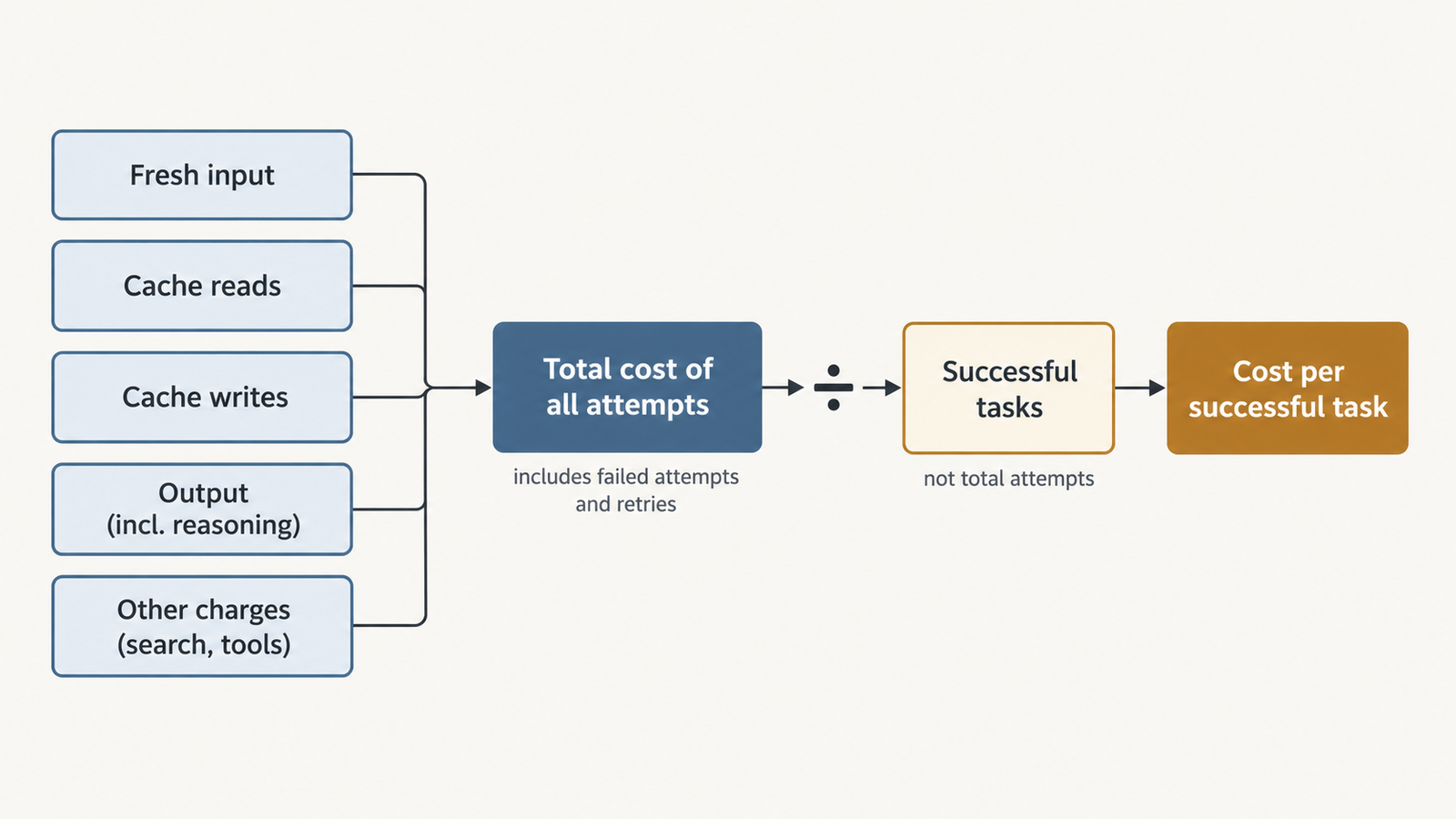
Last verified: 8 November 2026. Both papers are unreviewed working papers, and no outside group has reproduced the results yet. No, AI did not break …
Model Distillation

Model Distillation Explained: When AI Learning Becomes Extraction

Last verified: 7 November 2026. Government and company claims are attributed throughout. None has been tested in court. A support team trains a small, cheap …

RAG vs Fine-Tuning: Which One You Actually Need

RAG vs fine-tuning

Take a support team that ships two prototypes on the same base model. The first searches the product documentation on every question and pastes the top passages into the prompt. The second was fine-tuned on 4,000 past tickets. In the demo, the fine-tuned one sounds better: right terminology, exact escalation format. Three weeks later pricing changes. The fine-tuned model keeps quoting the old plan; the retrieval system picks up the new page the morning it’s published.

Neither prototype failed at what it was built to do. Retrieval-augmented generation (RAG) changes what the model can see when it answers. Fine-tuning changes how the model behaves. So the RAG vs fine-tuning decision starts with a plain question: does your problem live in the facts, in the form of the output, or in both?

The short answer: start with RAG when answers depend on knowledge that changes, is large, or must be cited. Investigate fine-tuning when the model already knows enough but won’t reliably produce the format, style or task behaviour you need, and prompting hasn’t fixed it. Combine them only when you’ve measured both problems at once.

Key Takeaways
  • RAG updates knowledge at query time without touching weights. Fine-tuning is a weak, risky way to add facts: research found RAG consistently beat it for knowledge injection.
  • Fine-tuning earns its place on behaviour: output format, tone, classification and repeated specialised tasks, especially when it lets you shorten prompts.
  • RAG mostly costs you per query (retrieval plus extra input tokens); fine-tuning mostly costs you per update (data, training, evaluation, regression testing). Query volume and update frequency decide which is cheaper.
  • More retrieved text isn’t better. Models use information in the middle of long contexts less reliably, so retrieval precision beats retrieval volume.
  • Neither approach is a security boundary. Retrieved documents can carry injected instructions; training data can be poisoned.
  • A fine-tuned model is tied to its base model’s lifecycle. On OpenAI’s platform, tuned models are retired along with their base, so budget for re-tuning.

Quick Navigation


RAG vs Fine-Tuning: Two Different Ways to Change an AI System

The original RAG paper by Lewis and colleagues framed the distinction precisely. A model’s weights are parametric memory: knowledge absorbed in training, hard to inspect and hard to update. A searchable document index is non-parametric memory: knowledge the model reads at inference time. The authors pointed to two problems with parametric memory that retrieval helps with, providing provenance for an answer and updating what the model knows.

In a RAG system, the model doesn’t change. At query time the application embeds the question, searches an index, optionally reranks, and inserts the best passages into the prompt. Re-index an edited document and the next answer can reflect it.

Fine-tuning runs a training job on examples of the input and output you want, producing a modified set of weights or a small set of adapter weights. Parameter-efficient methods such as LoRA train a tiny fraction of the parameters (up to 10,000 times fewer than full fine-tuning of GPT-3 175B, the paper reports) without adding inference latency. That makes fine-tuning cheaper. It doesn’t make it a reliable way to store facts.

Five things get lumped together as “teaching the model”:

What needs to changeExampleUsual first tool
KnowledgeCurrent refund policy, a product’s API limitsRAG
BehaviourAsk a clarifying question before actingPrompting, then fine-tuning
StyleHouse tone, terminology, reading levelPrompting, then fine-tuning
Task formatFixed JSON schema, ticket triage labelsStructured outputs or prompting, then fine-tuning
Tool-use patternWhich tool to call, in what orderPrompting and tool definitions, then fine-tuning

Only the first row is about facts. The rest are about form, where fine-tuning has a real case.

RAG vs Fine-Tuning: What Changes When the Source of Truth Changes?

Most enterprise knowledge moves. Product documentation changes each release, policies are revised quarterly, manuals get errata, and support knowledge bases are edited daily. What matters is how often facts change and how quickly a wrong answer hurts.

RAG handles change by re-indexing, but it isn’t instant or automatic. A document edited at 09:00 isn’t retrievable until the ingestion pipeline has chunked, embedded and written it to the index. If the old version isn’t deleted, both can be retrieved and blended. Two sources that disagree, such as a policy page and an outdated FAQ, produce an answer that cites one and contradicts the other. These are data-engineering problems: freshness targets, deletion handling, versioning and source precedence.

Fine-tuning handles change by retraining, and that’s the core reason it’s rarely the first choice for factual knowledge. Ovadia and colleagues compared the two for knowledge injection and found that RAG consistently outperformed unsupervised fine-tuning, for knowledge the model had seen before and for entirely new facts. They also found models struggled to learn new facts this way unless exposed to many variations of each one. A separate study by Gekhman and colleagues found that fine-tuning examples containing new knowledge are learned much more slowly than familiar ones, and that once learned they increase the model’s tendency to hallucinate. Their conclusion: models acquire facts mainly in pre-training, and fine-tuning mostly teaches them to use what they already know.

That doesn’t rule fine-tuning out of fast-changing domains. A claims assistant might retrieve current policy wording while a fine-tuned model handles the stable part: extracting fields into a fixed schema and flagging exceptions consistently. The facts live outside the model; the behaviour lives inside it.

RAG vs Fine-Tuning Cost: The Cost of a Query Versus the Cost of an Update

RAG is cheap to change and pays on every query. Fine-tuning pays each time something changes and can be cheaper per query.

  • RAG costs fall into fixed and variable parts. Fixed: preparing documents, building the chunking and embedding pipeline, search infrastructure and re-indexing. Variable, per query: embedding the question, the search, any reranking and, usually the largest line, the extra input tokens from retrieved passages. Evaluation and monitoring sit on top.
  • Fine-tuning costs are weighted the other way. Fixed: curating training examples, training jobs, experiments, evaluation against a baseline and, on every refresh, retraining, regression testing, versioning and rollback. Variable: inference on the tuned model, which may be priced differently from the base model or need dedicated serving if self-hosted.

One fixed cost is easy to miss: a fine-tune is bound to its base model. OpenAI’s fine-tuning guide, checked on 25 October 2026, says the platform is being wound down and closed to new users; existing customers can train until 6 January 2027, and tuned models last only as long as their base model. Whatever your provider, budget for re-tuning and re-evaluating when the base model retires.

A break-even model

Define, over one evaluation period:

  • Q = number of queries
  • C_R = fixed RAG setup and maintenance cost
  • V_R = average variable RAG cost per query
  • C_F = fixed fine-tuning, evaluation and maintenance cost
  • V_F = average variable cost per query on the fine-tuned model

Then:

Total RAG cost = C_R + Q × V_R

Total fine-tuning cost = C_F + Q × V_F

When fine-tuning has the higher fixed cost (C_F > C_R) and the lower per-query cost (V_F < V_R), the volume at which the two totals are equal is:

Q* = (C_F − C_R) / (V_R − V_F)

Below Q*, RAG is cheaper; above it, fine-tuning is. If V_F isn’t lower than V_R, for instance because a tuned model’s per-token premium outweighs the context saved, fine-tuning never breaks even on cost.

Most of the gap V_R − V_F usually comes from context. If fine-tuning lets you drop T_ctx retrieved tokens from every prompt at an input price of P_in per token, then V_R − V_F is roughly T_ctx × P_in plus the retrieval cost, minus any premium the tuned model charges per token. OpenAI’s optimisation guide makes the same point from the other side: fine-tuning can allow shorter prompts with fewer examples and less context, saving tokens at scale. That saving only exists if the facts you were retrieving can be dropped, which is rarely true for changing knowledge.

Three assumptions limit the model. It’s only valid if both systems meet the same quality, latency, security and availability targets. C_F recurs with every data refresh, so frequent updates multiply it. And it ignores the cost of being wrong. Add an error term, with p as the share of answers that are wrong and K as the average cost of a wrong answer (a refund, an escalation, a compliance review), and each total gains Q × p × K. A cheaper system with a higher error rate can cost more overall. UniverseBlend’s breakdown of what inference actually costs per token covers how request shape, caching and batching change V in practice.

RAG vs fine-tuning

Context Length and Inference Latency in RAG vs Fine-Tuning

Every retrieved passage is input the model must process before it writes the first token. That prefill work grows with prompt length, so retrieval adds to time-to-first-token as well as cost. Generation speed changes less with context length than the wait before it starts.

More context also isn’t more accuracy. Liu and colleagues found that models used relevant information best when it sat at the beginning or end of the input and noticeably worse when it sat in the middle, even for models built for long contexts. Retrieving the top 20 chunks “to be safe” can push the one that matters into exactly that position.

The levers are about precision: chunks sized to the unit of meaning (a policy clause, an API endpoint), a reranker that cuts a wide search to a few passages, and compression of long sources. UniverseBlend’s piece on context engineering in AI agents covers how ordering and caching stable prompt sections cut cost and latency, which applies directly to RAG prompts.

Fine-tuning doesn’t make context unnecessary. A tuned model still needs today’s facts, the user’s details and any document it’s asked about. What it can remove is scaffolding: long instructions and few-shot examples that taught the format. That saving is real at high volume, and different from dropping retrieved knowledge.

RAG vs Fine-Tuning: Accuracy, Evaluation and Failure Modes

The two architectures fail in recognisably different ways, and a fluent answer can hide either.

RAG fails when retrieval misses the right passage, the index holds stale or wrong documents, chunk boundaries split the sentence that mattered, the reranker drops key evidence, or the model answers beyond what the text supports. The last is hardest to spot, because the answer arrives with citations.

Fine-tuning fails when training examples are inconsistent (the model learns the errors), when it overfits and handles new inputs worse, when it regresses on abilities the base model had, and when teams assume training on a document means the model will recall it. The Gekhman results suggest that assumption can worsen hallucination.

Evaluate both on a representative test set drawn from real queries, not on demo prompts. For RAG, measure retrieval separately from generation: were the right passages retrieved (recall at k), was the set focused, and was the answer faithful to it? The Ragas framework evaluates these dimensions without human labels for every case. For both, measure correctness, task success, latency and cost per query, and rerun a regression suite on every index rebuild or model version.

RAG vs Fine-Tuning: Security and AI Agent Implications

Retrieval puts external text into the model’s context, and the model can’t reliably tell data from instructions. Greshake and colleagues showed attackers could plant prompts in content an application was likely to retrieve and steer its behaviour and tool calls. In an agent, a poisoned wiki page is an attack path.

Fine-tuning carries a different risk: a model trained on poisoned data carries the problem into every answer, and editing a document won’t fix it. The OWASP Top 10 for LLM Applications 2025 lists both, as prompt injection (LLM01) and data and model poisoning (LLM04), alongside vector and embedding weaknesses (LLM08), which covers retrieval stores themselves.

Neither architecture is a security boundary. Fine-tuning doesn’t reliably train away injection, and phrase filters are easy to evade. The controls that hold sit outside the model: permission-aware retrieval so users only retrieve what they’re allowed to read, provenance on every indexed document, access controls on the index, least-privilege tool permissions and confirmation for irreversible actions. UniverseBlend’s analysis of how agent prompt-injection benchmarks score failures explains why passing a benchmark isn’t proof of safety.

The Facts–Form–Frequency Test: A RAG vs Fine-Tuning Decision Framework

The Facts–Form–Frequency test, developed for this article rather than an industry standard, splits each requirement in two and asks how often each part changes.

  • Facts: what the model must know that it doesn’t reliably know now.
  • Form: how the output must look or behave, consistently.
  • Frequency: how often each changes, and how many queries you’ll serve between changes.

The rules: changing facts go to retrieval. Form that prompting can’t hold goes to fine-tuning, once measured. Frequency and volume decide whether the fixed cost pays.

ScenarioRecommendationAssumption behind it
Frequently changing factual knowledgeRAGUpdates must appear within hours, not training cycles
Stable domain-specific output formatFine-tuning, after prompting and structured outputs fall shortThe format is consistent and examples are available
Repeated specialised task behaviourFine-tuningHigh volume, stable task, measurable gain over prompting
Large collections of reference documentsRAGCorpus too large for the context window and changing
Strict source attributionRAGAnswers must cite the passage they used
High-volume, predictable queriesEvaluate fine-tuning on costQ exceeds Q* at equal quality
Current facts and consistent behaviourBothBoth gaps measured separately
Base model already meets the barNeitherPrompting plus evals pass
RAG vs fine-tuning

When a Hybrid RAG and Fine-Tuning Architecture Makes Sense

A hybrid uses each method for what it’s good at. A fine-tuned extraction model returns contracts in a fixed schema while retrieval supplies the current clause library to check them against.

Hybrids cost more than either alone: you pay C_R and C_F, and a regression could come from the index or the model. Justify one with two measurements, a behaviour gap prompting didn’t close and a knowledge gap the tuned model alone didn’t close. Otherwise start with the simplest architecture that meets requirements, usually a strong base model with good prompting and retrieval.

RAG vs Fine-Tuning: A Workload-Based Implementation Checklist

A planning meeting should be able to answer these before committing:

  1. Baseline: What does the base model score on your test set with good prompting alone?
  2. Test data: Do you have a few hundred real, labelled queries, including hard and adversarial ones?
  3. Update frequency: How often do the underlying facts change, and how stale may an answer be?
  4. Volume: What’s Q per month now and in a year, and what are C and V for each option?
  5. Cost: Are you logging input tokens, retrieval calls and cost per successful task?
  6. Latency: What time-to-first-token and end-to-end targets must hold at peak?
  7. Security: Who may retrieve which documents, which tools can the model call, and what needs human confirmation?
  8. Rollback: Can you revert an index build or model version in minutes?
  9. Lifecycle: When does your base model retire, and who re-tunes and re-tests on its replacement?
  10. Monitoring: Which drop in recall, faithfulness, task success or cost triggers review?

Conclusion

Start with RAG when answers depend on changing facts, a large corpus or a citation requirement. Investigate fine-tuning when the base model knows enough but won’t hold a format, style or task behaviour at your volume after proper prompting. Use both only when you’ve measured both gaps.

The useful next step is small: take 200 real queries, run them through the base model with good prompting, and label every failure as a facts problem or a form problem. The split tells you which approach to build first.

FAQ

Is RAG better than fine-tuning?

Neither in general. RAG suits current or large bodies of knowledge; fine-tuning suits consistent behaviour and format.

Can RAG and fine-tuning be used together?

Yes: a fine-tuned model for task format plus retrieval for current facts. It’s worth the extra cost only when both gaps are measured.

Is RAG cheaper than fine-tuning?

Not always. RAG has lower fixed costs but adds cost to every query; fine-tuning can win at high volume if it removes context, but every update adds fixed cost.

Does fine-tuning add new knowledge to an LLM?

Unreliably. Models learn new facts slowly this way, and learning them can increase hallucination.

Does RAG increase token usage?

Yes. Retrieved passages are extra input tokens on every query. Tighter retrieval and reranking reduce the increase.

Which approach is better for frequently changing information?

RAG. Updating an index takes minutes to hours; updating weights takes a training cycle plus evaluation.

Can fine-tuning improve structured output?

Often. Try structured-output features and prompting first, then fine-tune if format errors persist at your volume.

Does RAG make an AI agent more secure?

No. Retrieved documents can carry prompt injections. Security comes from permissions, provenance and tool controls outside the model.


Keep reading

Anthropic IPO valuation

Anthropic IPO: The $895 Billion Question Behind Its Valuation

Last updated: 9 November 2026. Latest confirmed development: Anthropic’s amended S-1, filed on 2 November, still leaves the share count and the IPO price range …
Claude Opus vs Sonnet

Claude Opus vs Sonnet: What the 2026 Price Gap Actually Buys

Last verified: 8 November 2026. All prices are Anthropic’s standard first-party API rates in US dollars per million tokens. They aren’t Claude Pro or Max …
RSA-1024

Did AI Break RSA? What DeepMind Actually Found
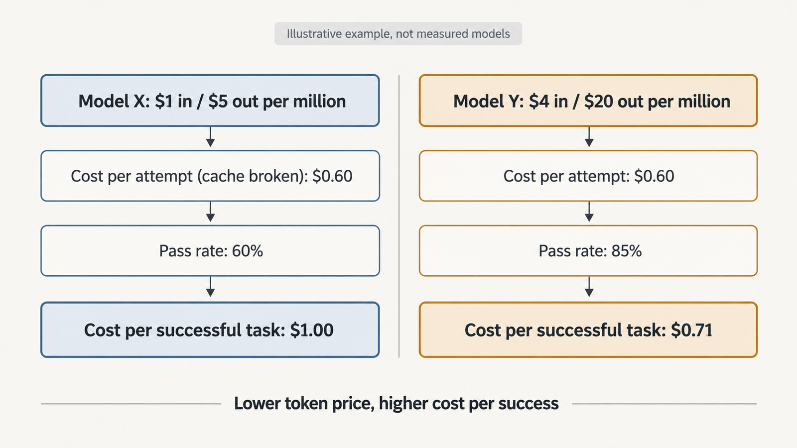
Last verified: 8 November 2026. Both papers are unreviewed working papers, and no outside group has reproduced the results yet. No, AI did not break …
Model Distillation

Model Distillation Explained: When AI Learning Becomes Extraction

Last verified: 7 November 2026. Government and company claims are attributed throughout. None has been tested in court. A support team trains a small, cheap …