LLM Context Window Comparison 2026: Limits and Costs

LLM context window

Specifications and prices checked October 11, 2026 · Prices in USD per million tokens, standard API tier

Short answer: In an LLM context window comparison for 2026, input capacity barely separates the leading models. Every proprietary API checked here accepts about 1 million tokens (1M to 1,050,000), and the two open-weight hosts list 1M or 524,288. Output caps differ more, from 65,536 tokens on Gemini to 128,000 on GPT-6.1 Sol and Claude Opus 5.5. Long-context pricing rules differ most of all: a 300,000-token prompt costs anywhere from $0.06 to $1.20 in input charges.

Three numbers get conflated in most spec sheets. The context window is how much a model can read in one request. The output limit is how much it can write back. The long-context pricing threshold is the prompt size at which the provider starts charging more. A model can have a huge window, a modest output cap and a threshold that doubles your bill well before you get near the window’s edge.

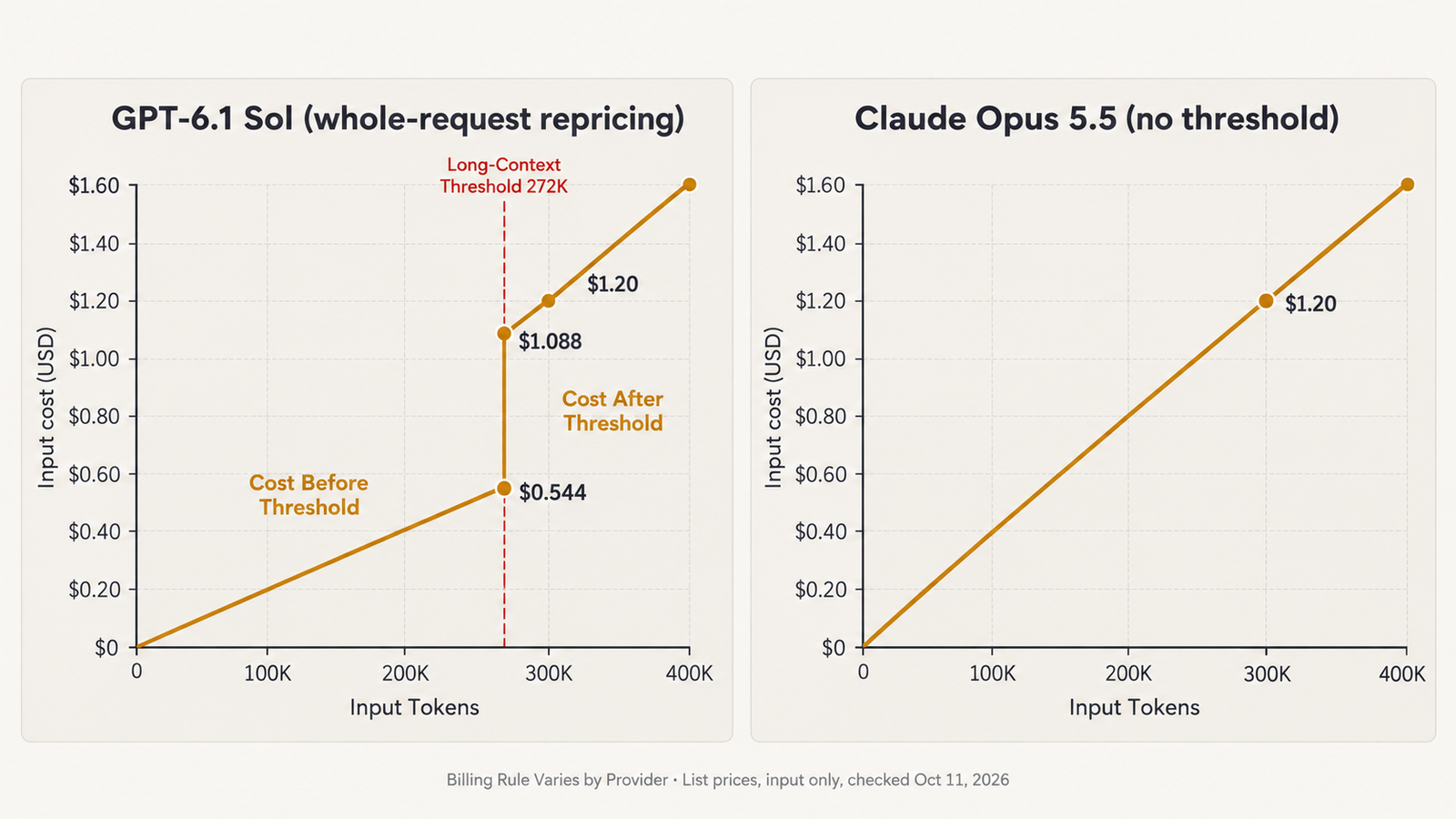
The third number is the one buyers skip. GPT-6.1 Sol charges $2.00 per million input tokens up to 272,000 tokens and $4.00 per million above it, and OpenAI applies the higher rate to the full request. A 270,000-token prompt costs $0.54. A 280,000-token prompt costs $1.12. Ten thousand extra tokens cost 58 cents.

Key Takeaways
  • Context capacity has converged. Every proprietary model checked lists about 1M input tokens, so window size rarely decides a purchase in 2026.
  • Output caps have not converged. Gemini 3.1 Pro and 3.8 Flash cap output at 65,536 tokens, about half of GPT-6.1 Sol’s and Claude Opus 5.5’s 128,000.
  • Three providers reprice by prompt size. OpenAI does it above 272K for the whole request, Google above 200K for Gemini 3.1 Pro, and Anthropic above 100K for Claude Haiku 5.5 only.
  • Claude Opus 5.5 and Sonnet 5.5 have no long-context surcharge. At 300K tokens, Opus 5.5 ($1.20) costs the same as GPT-6.1 Sol and Gemini 3.1 Pro, even though its base rate is twice theirs.
  • Crossing a threshold can cost more than the extra tokens are worth. Just past 272K, a GPT-6.1 Sol prompt more than doubles in price.
  • Caching flattens the comparison. A fully cached 300K prefix costs $0.06 on both GPT-6.1 Sol and Claude Opus 5.5.
  • Open-weight hosting is cheapest per token, but a host’s served context can differ from the model card. Check the endpoint, not the paper.

Quick Navigation


The LLM context window comparison table

All values are taken from official documentation and were checked October 11, 2026. “Threshold” is the prompt size at which input pricing changes. Costs cover input tokens only, with no output, caching, batch discounts or taxes.

Model and versionMax input contextMax outputLong-context thresholdInput belowInput above300K input costAvailabilityDocumentation
GPT-6.1 Sol (gpt-6.1-sol)1,050,000128,000>272K, whole request$2.00$4.00$1.20GA, OpenAI APIModel page
GPT-6 Luna (gpt-6-luna)1,050,000128,000>272K, whole request$0.10$0.20$0.06GA, OpenAI APIModel page
Claude Opus 5.5 (claude-opus-5-5)1M128,000None$4.00n/a$1.20Current, Claude APIModels · Pricing
Claude Sonnet 5.5 (claude-sonnet-5-5)1M128,000None$2.00n/a$0.60CurrentSame as above
Claude Haiku 5.5 (claude-haiku-5-5)1M128,000>100,000$0.10$0.50$0.15CurrentSame as above
Gemini 3.1 Pro (gemini-3.1-pro-preview)1,048,57665,536>200K$2.00$4.00$1.20PreviewModel · Pricing
Gemini 3.8 Flash (gemini-3.8-flash)1,048,57665,536None$0.75 (to Dec 31, 2026; $1.50 from Jan 1, 2027)n/a$0.225StableModel
Gemini 3.5 Flash-Lite (gemini-3.5-flash-lite)1,048,57665,536None$0.30n/a$0.09StableModel
Mistral Large 4 (mistral-large-4)1MNot publicly documentedNone documented$0.68 sale ($1.36 list)n/a$0.204 salePublic Preview, open-weightModel page
Llama 4 Maverick (Together AI)1M per model card; host lists 1,048K and 524,288Not publicly documentedNone documented$0.27n/a$0.081Hosted endpointModel card · Host
Qwen3.8-2.4T-A95B (Together AI)262,144 native; 1M served131,072None documented$2.00n/a$0.60Hosted endpointModel card · Host

Whole-request rules apply where stated. OpenAI says prompts above 272K are “priced at 2x input and cache rates and 1.5x output for the full request.” Anthropic says a Haiku 5.5 request over 100,000 tokens “pays the higher prices,” counting cache reads and writes toward prompt length. Google’s table selects the rate by prompt size (“prompts > 200k tokens”) but does not explicitly say the whole prompt is repriced. This article assumes it is, and that is an interpretation of Google’s wording.

The open-weight rows describe one host’s endpoint, not the model. Qwen3.8’s model card gives 262,144 tokens natively, extensible to about 1M. A 300K request on Together therefore runs in the extended range, where quality can differ from native-length behaviour.

Context window versus output limit

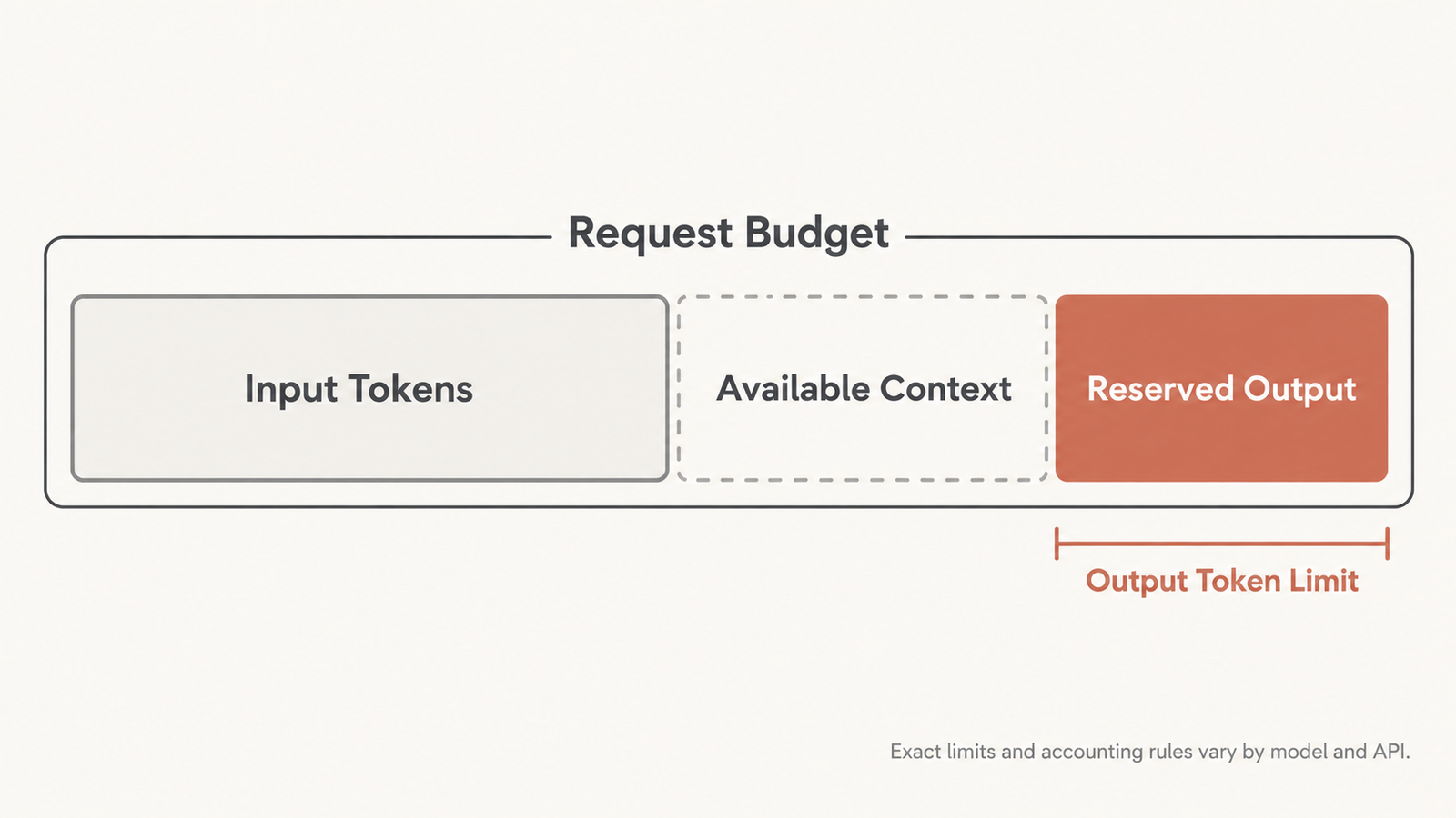
The context window caps what goes in. The output limit caps what comes out in a single response. They are documented separately for every proprietary model here, and they constrain different workloads.

Output limits bind harder than input limits. A model that reads a 400-page contract can only write 65,536 tokens back if it is Gemini 3.1 Pro, or 128,000 if it is GPT-6.1 Sol or Claude Opus 5.5. That is roughly 50,000 versus 100,000 words, before any reasoning tokens. Google bills thinking as output (“output price including thinking tokens”), so whether reasoning also draws on the output cap matters for long reasoning tasks. Check each provider’s documentation for that point, because accounting differs.

Some providers also treat input and output as one shared budget, so a large prompt leaves less room to answer. Qwen’s model card illustrates the general point: it recommends allowing 262,144 tokens for reasoning and 131,072 for the final answer, figures that only make sense if the request budget is planned as a whole.
LLM context window

Where long-context pricing start

Three of the providers checked charge more once a prompt gets long. Each draws the line in a different place and handles it a little differently.

  • OpenAI, 272K, whole request. For GPT-6.1 Sol and GPT-6 Luna, prompts above 272K input tokens pay double the input and cache rates and 1.5 times the output rate, on every token in the request. OpenAI’s pricing page lists the long-context column, and the threshold and the “full request” rule appear on each model page.
  • Google, 200K, by prompt size. Gemini 3.1 Pro charges $2.00 input and $12.00 output for “prompts <= 200k tokens”, and $4.00 and $18.00 for larger prompts. Context caching moves from $0.20 to $0.40. Gemini 3.8 Flash and 3.5 Flash-Lite have no split.
  • Anthropic, 100K, Haiku only. Anthropic’s pricing documentation states that its current models other than Claude Haiku 5.5 “include the full 1M token context window at standard pricing”, adding that “a 900k-token request is billed at the same per-token rate as a 9k-token request.” Haiku 5.5 moves from $0.10 to $0.50 per million input tokens above 100,000 prompt tokens, a fivefold jump, and cache reads count toward that total.

Mistral and the two open-weight hosts publish no threshold.

One ambiguity matters for anyone sizing prompts close to a boundary. Neither OpenAI nor Google says whether “272K” or “200K” means thousands or multiples of 1,024 tokens. The calculations below avoid the gap by testing well clear of either reading.

What a 300K-token request costs

The scenario: one request with 300,000 input tokens, zero output and no caching. It isolates the input-side effect of each pricing rule. These are author calculations from the official prices above, in USD.

Formula, where the provider reprices the whole request once a prompt crosses threshold T:

\text{Input cost} = \frac{N}{1{,}000{,}000} \times \begin{cases} r_{\text{standard}} & N \le T \\ r_{\text{long}} & N > T \end{cases}
Just below and just above each threshold
ModelBelow thresholdCostAbove thresholdCostJump
GPT-6.1 Sol270,000 tokens$0.540280,000 tokens$1.120+$0.58 for 10K more tokens
GPT-6 Luna270,000$0.027280,000$0.056+$0.029
Gemini 3.1 Pro190,000$0.380210,000$0.840+$0.46 for 20K more tokens
Claude Haiku 5.599,000$0.0099101,000$0.05055.1x for 2% more tokens
At 300,000 tokens
ModelRate applied300K input cost
GPT-6.1 Sol$4.00 (long-context)$1.20
Claude Opus 5.5$4.00 (standard)$1.20
Gemini 3.1 Pro (preview)$4.00 (long-context, assumed whole prompt)$1.20
Claude Sonnet 5.5$2.00$0.60
Qwen3.8-2.4T-A95B on Together$2.00$0.60
Gemini 3.8 Flash$0.75 (2026 rate)$0.225
Mistral Large 4 (preview)$0.68 sale / $1.36 list$0.204 / $0.408
Claude Haiku 5.5$0.50 (long-context)$0.15
Gemini 3.5 Flash-Lite$0.30$0.09
Llama 4 Maverick on Together$0.27$0.081
GPT-6 Luna$0.20 (long-context)$0.06

The three-way tie at the top is the central finding. On list prices, Claude Opus 5.5 costs twice as much as GPT-6.1 Sol per input token. At 300K tokens, OpenAI’s threshold has already doubled Sol’s rate and Google’s has doubled Gemini 3.1 Pro’s, while Opus stays flat. All three land at $1.20. Below 200K, Opus costs twice as much as either. Above 272K, the gap disappears.

Separate scenario: adding an 8,000-token answer

Keep the 300K prompt and add 8,000 output tokens. OpenAI’s long-context rule raises Sol’s output rate to $15.00 per million, and Google’s raises Gemini 3.1 Pro’s to $18.00.

  • GPT-6.1 Sol: $1.20 + (8,000 / 1M × $15) = $1.32
  • Gemini 3.1 Pro: $1.20 + (8,000 / 1M × $18) = $1.344
  • Claude Opus 5.5: $1.20 + (8,000 / 1M × $20) = $1.36
  • GPT-6.1 Sol at 270,000 input tokens instead: $0.54 + (8,000 / 1M × $10) = $0.62

Trimming 30,000 tokens from the prompt halves Sol’s bill. For Opus, the same trim saves about 9%.
LLM context window

Context window choices for RAG, coding and agents

  1. RAG pipelines. Retrieval systems control their own prompt size, which makes them the easiest place to exploit a threshold. A pipeline that routinely sends 250,000 to 300,000 tokens to GPT-6.1 Sol is paying the long-context rate on a share of requests that a retrieval cap of about 260,000 would remove. On Claude Opus 5.5 there is no such boundary to manage.
  2. Long-document analysis. Reading a large filing and returning a short summary is the case where big windows pay off most cleanly: input-heavy, output-light. The output cap rarely matters here, and the threshold often decides the bill.
  3. Coding agents. Consider an illustrative repository-aware agent that resends 300,000 tokens of code context on every turn. Without caching, 20 turns on GPT-6.1 Sol cost 20 × $1.20 = $24 in input alone. If the repository context is a stable prefix, OpenAI’s long-context cached rate of $0.20 per million drops each turn’s input to $0.06. That is why caching usually changes these comparisons more than the threshold does.
  4. Multi-agent systems. When several agents each carry a copy of a shared history, every copy is billed separately and pushed toward the threshold on its own. Summarising or pruning shared state before handoff can keep each call below a boundary that the combined history would cross.
  5. Long-running agents. Tool results accumulate. An agent that starts at 50,000 tokens and appends 10,000 per step crosses Gemini 3.1 Pro’s 200K line at step 16 and Sol’s 272K line at step 23. From that point every turn is billed at the higher rate. Compaction policies are cost controls, not just memory management.
  6. Prompt caching. Caching narrows the gap between providers on repeated context. At long-context rates, a fully cached 300K prefix costs $0.06 on GPT-6.1 Sol ($0.20 per million) and $0.06 on Claude Opus 5.5 ($0.20 per million cache hit). UniverseBlend’s earlier analysis of why a 50% price cut doesn’t halve agent bills made the same point for shorter contexts: once cache reads dominate, list-price gaps shrink. Note that Anthropic counts cache reads toward Haiku 5.5’s 100K threshold, and OpenAI doubles cache rates above 272K, so caching does not exempt a request from repricing.
  7. Splitting requests. Two 150,000-token GPT-6.1 Sol calls cost $0.60 in input, half the price of one 300,000-token call. That only works if the task decomposes. Cross-document reasoning does not split cleanly, and any shared instructions are paid twice. For Opus 5.5, splitting saves nothing on price.

A usable context budget is smaller than the advertised window. Rate limits measured in tokens per minute fill faster with long prompts, which UniverseBlend covered in AI API rate limits in 2026. This article makes no latency claims, but longer prompts add processing time before the first token.

A context window checklist before you choose

  • Measure your real prompt-size distribution, including p95, not just the average
  • Find each candidate’s threshold and whether it reprices the whole request
  • Check the output cap against your longest required answer, including reasoning tokens
  • Price the workload with your actual cache-hit rate
  • Confirm the hosted endpoint’s served context for open-weight models, not just the model card
  • Note preview status (Gemini 3.1 Pro, Mistral Large 4) and dated price changes (Gemini 3.8 Flash on January 1, 2027)
  • Check tokens-per-minute limits at your prompt size
  • Test quality at your real context length; a model accepting 1M tokens says nothing about how well it uses them

Conclusion

This LLM context window comparison shows the window itself has stopped being a differentiator. Nearly everything accepts about a million tokens. What separates the models is the output cap, whether the model is still in preview, and above all the pricing rule waiting at 100K, 200K or 272K tokens.

For workloads that sit under 200K tokens, list prices are a fair guide. For workloads that regularly cross 272K, a model with no surcharge can match one with half its base rate, and trimming a prompt by 10% can halve the bill. Price your real prompt distribution against each provider’s rule before trusting the headline number.

Frequently Asked Questions

What is the difference between an LLM context window and an output token limit?

The context window is the maximum input a model accepts in one request. The output limit is the maximum it can generate in one response. As of October 2026, most leading models accept about 1M input tokens, but output caps range from 65,536 (Gemini) to 128,000 (GPT-6.1 Sol, Claude Opus 5.5).

Does a larger context window always mean a better model?

No. Capacity says nothing about how well a model uses long context, and the largest windows now look nearly identical across providers. Output limits, pricing thresholds and quality at your real prompt length matter more.

What happens when a request exceeds the context window?

The API generally rejects it or requires you to shorten the input. Exact error behaviour varies by provider. Applications should count tokens before sending and trim, summarise or split oversized inputs.

How does long-context pricing work?

Some providers charge a higher per-token rate once a prompt passes a set size. In October 2026 that meant 272K for OpenAI’s GPT-6.1 Sol and GPT-6 Luna, 200K for Google’s Gemini 3.1 Pro, and 100K for Anthropic’s Claude Haiku 5.5. Claude Opus 5.5 and Sonnet 5.5 have no surcharge.

Does crossing a pricing threshold reprice the entire request?

For OpenAI, yes: the documentation says the higher rates apply “for the full request.” Anthropic’s Haiku 5.5 rule also applies the higher price to any request over the threshold. Google selects the rate by total prompt size but does not state the whole-request rule as explicitly.

Can prompt caching reduce long-context costs?

Yes, often by more than avoiding a threshold. A fully cached 300K prefix costs $0.06 on GPT-6.1 Sol or Claude Opus 5.5, against $1.20 uncached. Caching does not exempt a request from long-context repricing, though.

How should developers compare proprietary and open-weight models?

Compare the specific hosted endpoint, not the model card. A host may serve a different context length than the paper describes. Qwen3.8’s native 262,144-token context is extended to 1M on Together AI, for example.

What should an AI agent developer measure before choosing a model?

Prompt-size growth per step, the step at which each provider’s threshold is crossed, output needs per turn, cache-hit rate and tokens-per-minute limits. Then test answer quality at the context length the agent actually reaches.


Keep reading

Types of AI Models

Types of AI Models in 2026: A Field Guide From LLMs to World Models

Model details checked against official announcements, model cards and documentation on 1 November 2026. Line up four AI models that were current at the end …
AI Coding Agent

AI Coding Agents Are Getting Expensive. Who’s Paying for the Tokens?

Pricing checked on official vendor pages on 1 November 2026. All USD. Cost scenarios are illustrative and labelled as such. On 28 October, TechCrunch published …
generative AI architecture

Generative AI Architecture: The 7 Layers That Are Hard to Undo

Published 30 October 2026. API prices checked 28–30 October 2026 on each provider’s official pricing page. Cost figures below are labelled as illustrative where they …
Indirect Prompt Injection

Gemini 4 Carbon Hit 0% on Indirect Prompt Injection. Is That Enough?

When Google announced Gemini 4 Carbon on 28 October, one line in the safety section stood out. Carbon scored 0.0% on Gray Swan’s Indirect Prompt …

LLM Inference Latency by Model and Provider: Real Numbers

LLM inference latency

Published October 2026 · Data read October 11, 2026 · Source: Artificial Analysis provider benchmarks, secondary research

The same open-weight model, Llama 3.3 70B, starts answering in 0.67 seconds on Google Vertex and 2.37 seconds on DeepInfra. Once it starts, Groq streams 328 tokens per second and DeepInfra 17. A 500-token answer takes 2.4 seconds on Groq and 32.5 seconds on DeepInfra’s FP8 “Turbo” endpoint.

Those figures come from Artificial Analysis, which runs the same 10,000-token prompt against every host from one Google Cloud VM in Iowa and reports the median over 72 hours. That is about as fair as public LLM inference latency data gets, and it is still not perfectly fair. DeepInfra’s endpoint is quantized to FP8, no host discloses its hardware or batch size, and a request from Frankfurt or Mumbai will see different network time.

The spread is the point. Rate limits tell you how much a provider lets you run, and pricing tells you what it costs. Latency decides whether the product feels usable. That depends far more on the serving stack and the settings you choose than on the model’s name.

Key Takeaways
  • For one model, host choice moved output speed 19-fold (17 to 328 tokens/s for Llama 3.3 70B) and time to first token 3.5-fold.
  • Reasoning effort dominates frontier-model latency. On Artificial Analysis’s default “max” setting, Claude Sonnet 5.5 took about 490 seconds to its first answer token. Its low setting is listed at under a second on the provider leaderboard, a figure to check before quoting.
  • Time to first token (TTFT) and output speed are separate problems. A short chat reply is dominated by TTFT. A long report is dominated by output speed.
  • Agents multiply latency. Five sequential calls on a slow endpoint can take more than 100 seconds before tool time is added.
  • Published medians hide tail latency. No source examined here published p95 figures, so you have to measure them yourself.
  • Test with your own prompt lengths, region and reasoning settings before trusting any ranking, including this one.

Quick Navigation


Why LLM inference latency is hard to compare

Two published numbers for “the same model” can differ for at least six reasons that have nothing to do with the model: where the test client sits, how long the prompt is, how many requests run at once, which reasoning setting is on, how the host quantizes and batches, and which statistic is reported.

Even one careful source can disagree with itself. On Artificial Analysis’s Gemini 3.5 Flash-Lite page, the headline gives 414 tokens per second and the comparison table gives 365. Its GPT-6.1 Sol page reports a time to first answer token of 311 seconds in the headline and 327 seconds in the table. Neither page explains the gap. Different averaging windows are the likely cause, but that is an inference, not a documented fact. If a single benchmark cannot hold one number steady across its own page, rankings stitched together from several sources deserve more suspicion.

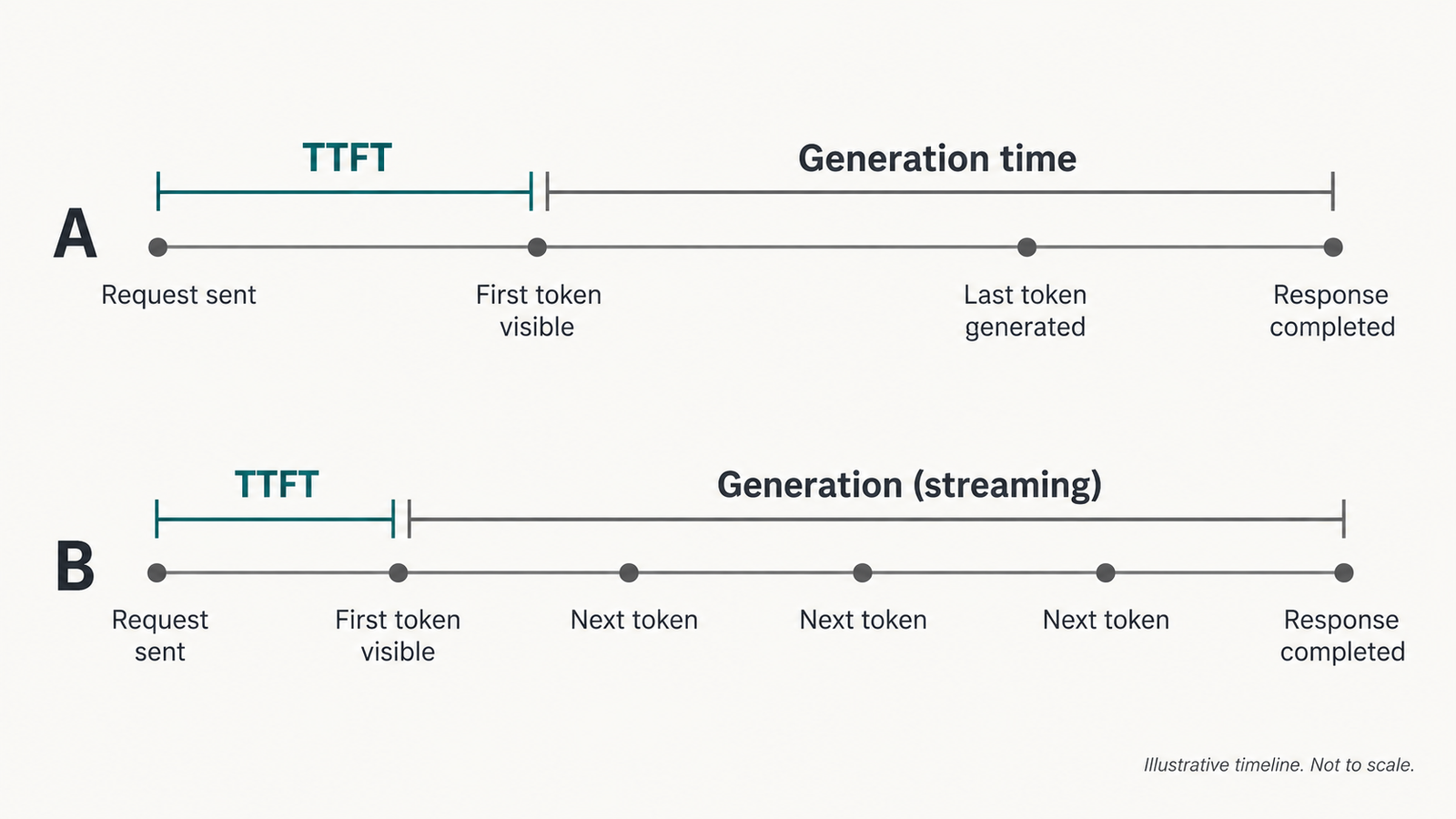
What TTFT actually measures

Time to first token (TTFT) is the wall-clock time between sending a request and receiving the first token of the response. Artificial Analysis’s methodology defines it that way and measures from the client.

That single number folds together several stages:

  • network time from client to provider and back
  • admission and queueing behind other customers’ requests
  • prefill, where the model processes the entire prompt before it can generate anything
  • any provider-side orchestration, such as safety checks, routing or tool-schema handling
  • for reasoning models, the thinking phase, if the measurement waits for the first answer token

Providers do not publish this breakdown, and a client-side measurement cannot separate the stages. A slow TTFT could mean a long queue, a long prompt or a distant data centre.

The reasoning point causes most of the confusion. Artificial Analysis reports two variants: TTFT to the first token of any kind, and “time to first answer token”, which includes thinking. Its per-model pages for frontier models use the second variant. That is why Claude Opus 5.5 at max effort shows roughly 600 to 1,000 seconds depending on host. The figure measures how long the model chose to think, not how fast Anthropic, Google, Azure or Amazon serve it.

TTFT versus output tokens per second

Output speed is the average rate at which tokens arrive after the first one. Artificial Analysis defines it as tokens received per second after the first token. It governs how long a full answer takes. TTFT governs how long the user stares at nothing.

The two do not move together. On Llama 3.3 70B, Google Vertex had the lowest TTFT (0.67 s) but streamed at 162 tokens/s, while SambaNova was slower to start (2.26 s) but generated faster (280 tokens/s). For a 50-token reply, Vertex wins comfortably. For a 2,000-token document, SambaNova finishes first.

The gap comes from different bottlenecks. Prefill is mostly compute-bound, processing many prompt tokens in parallel. Decode, the token-by-token generation that follows, is mostly limited by memory bandwidth, because the model’s weights stream through the chip for every token. Hardware and batching choices that help one phase can hurt the other. Large batches raise a provider’s total throughput but slow each individual stream.

LLM inference latency

LLM inference latency by model and provider

All figures are third-party measurements by Artificial Analysis, read October 11, 2026. Conditions throughout: about 10,000 input tokens, single request at a time, client in Google Cloud us-central1-a, streaming, median of the previous 72 hours. “End-to-end” is the time to receive a 500-token answer. None of this was measured by UniverseBlend.

Table 1: One model, many hosts (the controlled comparison)
ModelHostTTFT (s)Output speed (tok/s)End-to-end, 500 tokens (s)Notes
Llama 3.3 70BGoogle Vertex0.671623.76Precision not reported
Llama 3.3 70BGroq0.853282.37Custom LPU hardware
Llama 3.3 70BCoreWeave0.89787.34Not reported
Llama 3.3 70BScaleway1.48738.34Headline TTFT 1.34 s
Llama 3.3 70BTogether AI (Turbo)1.59718.65“Turbo” variant
Llama 3.3 70BNovita1.784512.83Not reported
Llama 3.3 70BAzure2.241216.38Not reported
Llama 3.3 70BSambaNova2.262804.05Headline speed 294.5
Llama 3.3 70BDeepInfra (Turbo)2.371732.53FP8
Llama 3.3 70BParasail2.57868.39FP8

Source: Artificial Analysis, Llama 3.3 70B providers. p95: not reported for any row.

Table 2: Frontier models at maximum reasoning effort
Model (API ID)HostTime to first answer token (s)Output speed (tok/s)End-to-end, 500 tokens (s)
Claude Sonnet 5.5 (claude-sonnet-5-5)Amazon475.97143479.46
Claude Sonnet 5.5Anthropic492.88142496.41
Claude Opus 5.5 (claude-opus-5-5)Google604.2595661.24
Claude Opus 5.5Anthropic704.1897667.28
GPT-6.1 Sol (gpt-6.1-sol)Azure288.6078294.99
GPT-6.1 SolOpenAI326.9456335.94

Sources: Artificial Analysis provider pages for Claude Sonnet 5.5, Claude Opus 5.5 and GPT-6.1 Sol. Effort: “max” with default fallback (Claude); “max” (GPT-6.1 Sol). These numbers mostly measure thinking time. Several Opus 5.5 rows show a time-to-first-answer longer than the 500-token total, an inconsistency the source does not explain.

Table 3: Lower-effort and lightweight endpoints (leaderboard view)
ModelHostFirst chunk (s)Output speed (tok/s)Total (s)Setting
Claude Sonnet 5.5Anthropic0.881005.86low effort
GPT-6 Luna (gpt-6-luna)OpenAI2.831256.84low effort
GPT-6.1 SolOpenAI2.804713.41low effort
Gemini 3.5 Flash-Lite (gemini-3.5-flash-lite)Google AI Studio8.9636510.33default; reasoning not reported
Qwen3.8 2.4T A95BTogether AI1.1411223.40not reported
Qwen3.8 2.4T A95BDigitalOcean0.825744.54not reported
Qwen3.8 2.4T A95BAlibaba Cloud2.993771.44not reported

Source: Artificial Analysis provider leaderboard, with Gemini from its model page. Treat this table as indicative: column values were extracted from a combined view and should be confirmed on the live page. The Qwen totals are high relative to their speed, which suggests reasoning output or longer answers. The source does not say which.

The Sonnet 5.5 rows across Tables 2 and 3 tell the main story. The same model on the same host goes from under one second to about eight minutes before answering, depending on a single API parameter.

Measurement-quality matrix
ComparisonSame model?Same harness?Same settings?Verdict
Llama 3.3 70B across hosts (Table 1)YesYesPrecision variesControlled; fair to rank, noting FP8 rows
One frontier model across clouds (Table 2)YesYesYes (max effort)Partially comparable; differences mix serving and thinking-time variance
Different frontier models (Table 2)NoYesEffort labels differ by vendorUnsuitable for a speed ranking; effort levels are not equivalent across vendors
Low-effort rows (Table 3)NoYesVariesIndicative only
Qwen across hosts (Table 3)YesYesNot reportedPartially comparable
Any of the above versus your own region and concurrencyn/aNoNoUnsuitable without retesting

How prompt length changes the first-token experience

Before a model can write its first word, it has to process every prompt token. More input means more prefill work, so TTFT generally rises with prompt length. Attention also scales worse than linearly with sequence length, which matters most at very long contexts.

In production the relationship is rarely clean. Providers split long prompts into chunks, interleave them with other customers’ work, and route long-context requests to different hardware. Artificial Analysis tests at 1,000, 10,000 and 100,000 input tokens for this reason. All the figures above use the 10,000-token workload, so they overstate TTFT for a short chat turn and understate it for a large retrieval prompt.

Caching changes the picture for repeated prefixes. Anthropic’s prompt-caching documentation says users “will generally see improved time-to-first-token for long documents” when a cached prefix is reused. Caching has no effect on output generation, and the default cache lives five minutes. The documentation gives no millisecond figure, so measure the gain on your own prompts.

Typical input sizeWhat to measure beyond the published median
Under 2,000 tokens (chat turns, classification)TTFT and first visible text from your own region; p95 under expected concurrency
2,000–30,000 tokens (RAG, documents)TTFT at three or more sizes in this range; cache-hit versus cache-miss TTFT
30,000+ tokens (codebases, long files)TTFT growth curve up to your real maximum; timeouts and error rate; whether the endpoint routes long prompts differently
Any size with a fixed system promptCached-prefix TTFT, and how quickly the cache expires under your traffic pattern

When streaming helps and when it does not

Streaming sends tokens as they are generated instead of waiting for the full response. It does not make the model faster. It changes when the user first sees something.

For a chat interface, that is often enough. Jakob Nielsen’s widely cited response-time limits, drawn from Miller (1968) and Card et al. (1991), put the edge of uninterrupted thought at about one second and the edge of sustained attention at about ten. A streamed answer that starts within a second and reads at a steady pace keeps a reader engaged, even if completion takes eight seconds.

Streaming fails in three common cases. The first is when the client needs the whole response before acting: structured JSON, a tool call or a function argument cannot be used half-written. The second is uneven cadence. Long pauses mid-stream, from server batching or client buffering in proxies and UI frameworks, can feel worse than a slightly later start. The third is reasoning models that show nothing until thinking ends, so a fast first token is meaningless if that token is hidden reasoning.

What LLM inference latency means for AI agents

This is where latency stops being a benchmark number and becomes a product problem. An agent rarely makes one call. It plans, calls a tool, reads the result and calls the model again, and every step pays TTFT and generation time in sequence.

A rough estimate per step:

T_{\text{step}} \approx \text{TTFT} + \frac{\text{output tokens}}{\text{output tokens per second}} + T_{\text{tool}}

This is an approximation. It ignores mid-stream pauses, retries and queueing spikes, and it assumes steps run one after another rather than overlapping.

The formula reproduces the source’s own totals. For Groq, 0.85 s + 500 / 328 tok/s = 2.37 s, exactly the published end-to-end figure. For DeepInfra, 2.37 + 500 / 17 = 31.8 s, against 32.5 s published.

Worked example (derived, not measured): a five-step agent, each step producing 300 output tokens and making one tool call that takes an assumed 0.8 seconds.

Endpoint (Table 1 or 2 figures)Per stepFive steps
Llama 3.3 70B on Groq0.85 + 0.91 + 0.8 = 2.56 s12.8 s
Llama 3.3 70B on Google Vertex0.67 + 1.85 + 0.8 = 3.32 s16.6 s
Llama 3.3 70B on DeepInfra (FP8)2.37 + 17.65 + 0.8 = 20.82 s104 s
Claude Sonnet 5.5, max effort, Anthropic492.88 + 2.11 + 0.8 = 495.8 sabout 41 minutes

The same five-step task is a 13-second interaction or a 41-minute background job, depending on host and settings. Neither outcome is wrong, but each implies a different product. Voice is stricter still: Stivers et al.’s 2009 PNAS study of turn-taking across 10 languages found average gaps between speakers clustering within 250 milliseconds of a cross-language mean. That points to a budget measured in hundreds of milliseconds, not seconds. That figure is a design guide drawn from human conversation, not a measured LLM threshold.

A reasonable set of engineering guidelines, labelled as such: aim for first visible text under about one second in chat, under a few hundred milliseconds of response gap in voice, and set an explicit end-to-end budget for agents, with p95 rather than median as the target.

LLM inference latency

Hosted APIs versus Llama and Qwen inference hosts

With a closed model, you can only buy latency from the vendor or the clouds that resell it. Table 2 shows that resellers can differ: GPT-6.1 Sol reached its first answer about 38 seconds sooner on Azure than on OpenAI’s own API, and streamed faster. With open weights you can also choose the serving stack, and Table 1 shows that choice matters more than anything else measured here.

That difference belongs to the host, not the model. Llama 3.3 70B is identical weights everywhere, yet output speed varies 19-fold. The causes are mostly undisclosed: accelerator type (Groq and SambaNova build their own chips), quantization (DeepInfra and Parasail are FP8), batch size and scheduling policy, and data-centre location relative to the test client. A slow host is not evidence that the model is slow, and a fast host’s numbers do not transfer to your own deployment.

Self-hosting gives you control of those variables and the responsibility for tuning them. It is also the economic question UniverseBlend examined in GPU Cloud Pricing 2026. Larger batches lower cost per token and raise per-request latency, so the cheapest configuration is rarely the most responsive one.

How to run a fair LLM inference latency test

No public benchmark matches your region, prompts and traffic. A minimal test you can run yourself:

  1. Run the client in the cloud region your users or servers actually use.
  2. Build prompts at your real input sizes, with three lengths minimum, and unique content per request so caching does not flatter results (then test cached prefixes separately).
  3. Fix output length with max_tokens and record the actual tokens returned.
  4. Set reasoning effort, temperature and tool schemas exactly as production will.
  5. Stream every request and timestamp each chunk on the client.
  6. Run at least a few hundred requests per configuration, spread across days and hours, at your expected concurrency.
  7. Report p50 and p95 for TTFT, inter-token gap and total time, plus the error and timeout rate.
import time

def measure(client, prompt, **settings):
    t0 = time.perf_counter()
    stamps = []
    for chunk in client.stream(prompt, **settings):   # provider SDK streaming call
        if chunk.text:                                  # ignore empty/keep-alive chunks
            stamps.append(time.perf_counter())
    ttft = stamps[0] - t0
    gaps = [b - a for a, b in zip(stamps, stamps[1:])]
    total = stamps[-1] - t0
    return {"ttft": ttft, "total": total,
            "max_gap": max(gaps, default=0),
            "chunks": len(stamps)}
# Run many times; report p50/p95 of each field, not the mean.

Chunks are not always single tokens, so divide counted output tokens by streaming time for a true rate. This sketch produces no results by itself, and none are reported here.

A practical provider selection framework

Pick metrics by workload before comparing providers.

CriterionMatters most whenHow to judge
TTFT at your input sizeChat, autocomplete, voicep95 from your region
Sustained output speedLong answers, reports, codeTokens per second after the first token
End-to-end completionAnything parsed as a whole (JSON, tools)p50 and p95 total time
VariabilityUser-facing productsGap between p50 and p95; largest mid-stream pause
Concurrency and rate limitsProduction trafficLatency at expected parallelism; see AI API rate limits in 2026
Tool-call overheadAgentsPer-step time multiplied by expected steps
Cost at required qualityAllCost per completed task at the reasoning setting you need

A single fastest-model ranking misleads in both directions. It can reward an endpoint that is fast because it thinks less, and penalise a model whose latency comes from a reasoning setting you would never use. Fix quality first, then compare latency among the options that meet it.

What the available evidence cannot tell us

The public data has clear gaps. It has no tail latency (medians only), one client location, mostly single-request load, and undisclosed hardware and batch sizes. Reasoning effort labels mean different things at different vendors. Frontier-model pages default to maximum effort, which few interactive products would use. Several source pages also show internal inconsistencies, so any figure here could shift by 10% or more when re-read. None of it tells you how a provider behaves during a regional incident or a demand spike, which is when latency matters most.

Conclusion

LLM inference latency becomes a product problem at a specific point: when the time a user or a downstream system must wait crosses the budget your interface was designed around. For chat that is roughly a second to first visible text. For voice it is hundreds of milliseconds. For agents it is the sum of every step, at the 95th percentile.

The evidence says the model name predicts that wait poorly. Host choice moved Llama 3.3 70B’s output speed 19-fold, and one reasoning parameter moved Claude Sonnet 5.5 from under a second to about eight minutes. Treat published rankings as a shortlist, then measure the two or three candidates yourself, with your prompts, in your region, at your load.

Frequently Asked Questions

What is a good LLM inference latency for a chatbot?

There is no universal standard. A common engineering guideline, based on Nielsen’s one-second limit for uninterrupted thought, is first visible text within about one second, with steady streaming after that. Measure p95, not just the median.

What is time to first token (TTFT)?

TTFT is the time from sending a request to receiving the first token of the response, measured at the client. It includes network time, queueing and prompt processing. For reasoning models it may also include thinking time, depending on whether the measurement waits for the first answer token.

Is TTFT or output tokens per second more important?

It depends on response length. Short replies are dominated by TTFT, and long documents by output speed. Estimate total time as TTFT plus output tokens divided by output speed for your typical response.

Why does the same open model have different latency on different hosts?

Hosts use different hardware, quantization, batching and data-centre locations. On Artificial Analysis’s October 2026 data, Llama 3.3 70B ran at 17 to 328 output tokens per second depending on host.

Why do reasoning models seem so slow in benchmarks?

Many benchmarks report time to the first answer token at the highest reasoning effort, which includes minutes of thinking. Lower effort settings respond in seconds. Compare models at the effort level you would actually use.

Does streaming reduce latency?

Streaming reduces the time until users see output, not the time to generate the full response. It helps chat, but does nothing for tool calls or structured output that must arrive complete.

Does prompt caching reduce latency?

It can reduce TTFT when a long prompt prefix repeats. Anthropic documents improved time-to-first-token for long cached documents and no effect on output generation speed. Gains depend on cache hits within the cache lifetime.

How do I benchmark LLM inference latency fairly?

Test from your production region, with your real prompt sizes and settings, streaming, at expected concurrency, over hundreds of requests across several days. Report p50 and p95 for TTFT and total time, plus errors.


Keep reading

Types of AI Models

Types of AI Models in 2026: A Field Guide From LLMs to World Models

Model details checked against official announcements, model cards and documentation on 1 November 2026. Line up four AI models that were current at the end …
AI Coding Agent

AI Coding Agents Are Getting Expensive. Who’s Paying for the Tokens?

Pricing checked on official vendor pages on 1 November 2026. All USD. Cost scenarios are illustrative and labelled as such. On 28 October, TechCrunch published …
generative AI architecture

Generative AI Architecture: The 7 Layers That Are Hard to Undo
Published 30 October 2026. API prices checked 28–30 October 2026 on each provider’s official pricing page. Cost figures below are labelled as illustrative where they …
Indirect Prompt Injection

Gemini 4 Carbon Hit 0% on Indirect Prompt Injection. Is That Enough?

When Google announced Gemini 4 Carbon on 28 October, one line in the safety section stood out. Carbon scored 0.0% on Gray Swan’s Indirect Prompt …

GPU Cloud Pricing 2026: What an Hour Actually Costs

GPU cloud pricing

Published: October 2026 · Pricing last verified: October 10, 2026. Provider pricing and availability may change; check the linked source before committing to a workload.

GPU cloud pricing for the same class of NVIDIA H100 runs from $2.89 per GPU-hour on RunPod (a single H100 PCIe pod) to about $11.68 per GPU-hour on Google Cloud, where an eight-GPU a3-megagpu-8g VM lists at $93.40 an hour. Prices were checked on October 10, 2026. That is a 4x spread for one chip, but the comparison is imperfect: the cheap end is one PCIe card with 16 vCPUs, the expensive end is a full SXM node with 3,200 Gbps of networking. Newer chips sit higher still, with NVIDIA B200 at $6.69 to $14.21 per GPU-hour depending on provider and billing model.

The more useful finding is that the hourly rate is the wrong number to optimise. On a published benchmark, the most expensive chip per hour produced the cheapest tokens.

Key Takeaways
  • On-demand H100 pricing spans $2.89 to $11.68 per GPU-hour across the providers checked; H200 runs $5.29 to $10.60 and B200 $6.69 to $8.60 where an on-demand rate is published.
  • Google Cloud now lists Ironwood (TPU7x) at $12.00 per chip-hour on demand in us-central1, falling to $5.40 on a three-year commitment. TPU chip-hours are not equivalent to GPU-hours.
  • Spot and commitment discounts are larger than most provider-to-provider gaps. CoreWeave’s spot H100 node costs 60% less than its on-demand rate.
  • Using MLPerf Llama 2 70B results, an eight-GPU B200 node produced output tokens for roughly $0.15 to $0.31 per million, against $0.41 to $0.64 for an H100 node. Throughput, not rental rate, set the winner.
  • Utilisation is the cost lever buyers underestimate. At 60% productive use, a $0.48 compute cost per million tokens becomes $0.83 once modest overhead is added.
  • Price your workload in cost per million output tokens at your realistic utilisation before comparing any two quotes.

Quick Navigation


The GPU cloud pricing comparison: H100, H200, B200 and TPU7x

Every figure below comes from the provider’s own pricing page, checked October 10, 2026. Where a provider sells only eight-GPU nodes, the per-GPU figure is the node price divided by eight, shown next to the original. US regions are used unless stated. Azure and AWS on-demand rates are the exception: both companies render prices in an interactive calculator, so those two rows rely on third-party mirrors of the official price APIs and are marked as such.

ProviderAcceleratorConfigurationOn-demandReserved / committedSpot / interruptibleRegion and conditionsVerifiedSource
RunPodH100 PCIe1 GPU pod, 80 GB, 16 vCPU, 188 GB RAM$2.89/GPU-hrQuote requiredNot verifiedPer-second billing; Community vs Secure tier not distinguished in page text2026-10-10RunPod pricing
RunPodH100 SXM1 GPU pod, 20 vCPU, 125 GB RAM$3.99/GPU-hrQuote requiredNot verifiedAs above2026-10-10RunPod pricing
LambdaH100 SXM8x instance, 208 vCPU, 1,800 GiB RAM$3.99/GPU-hr ($31.92/node)Quote requiredNot offeredSelf-serve, first come; plus sales tax2026-10-10Lambda pricing
AWSH100p5.48xlarge, 8 GPU$55.04/node ($6.88/GPU), via third-party mirrorCapacity Block $47.757/node ($5.97/GPU)Varies by zoneus-east-1; Capacity Blocks prepaid, price updates next January 20272026-10-10AWS Capacity Blocks
CoreWeaveH100HGX node, 8 GPU, 128 vCPU, 2 TB RAM$49.24/node ($6.16/GPU)Up to 60% off, quote required$19.71/node ($2.46/GPU)North America; egress free2026-10-10CoreWeave pricing
Google CloudH100a3-highgpu-8g, 8 GPU$88.49/node ($11.06/GPU)1-yr $61.38; 3-yr $38.86$50.32/nodeus-central1; spot price variable2026-10-10Google accelerator pricing
Google CloudH100a3-megagpu-8g, 8 GPU$93.40/node ($11.68/GPU)1-yr $64.21; 3-yr $40.65$53.10/nodeus-central12026-10-10Google accelerator pricing
AzureH100ND96isr H100 v5, 8 GPU$98.32/node ($12.29/GPU), via third-party mirrorNot verifiedNot verifiedEast US; official page renders client-side2026-10-10Azure VM pricing
RunPodH2001 GPU pod, 141 GB, 24 vCPU$5.29/GPU-hrQuote requiredNot verifiedInstant cluster rate $4.31/GPU-hr2026-10-10RunPod pricing
CoreWeaveH200HGX node, 8 GPU$50.44/node ($6.31/GPU)Quote required$20.93/nodeNorth America2026-10-10CoreWeave pricing
AWSH200p5e.48xlarge, 8 GPUNot verifiedCapacity Block $54.924/node ($6.87/GPU)Not verifiedUS East (Ohio), US West2026-10-10AWS Capacity Blocks
Google CloudH200a3-ultragpu-8g, 8 GPU$84.81/node ($10.60/GPU)1-yr $58.47; 3-yr $37.21$50.83/nodeus-central12026-10-10Google accelerator pricing
LambdaB200 SXM68x instance, 180 GB/GPU$6.69/GPU-hr ($53.52/node)1-Click Cluster, 2 wk–1 yr: $8.87–$9.86/GPU-hrNot offeredSelf-serve2026-10-10Lambda pricing
RunPodB2001 GPU pod, 180 GB, 28 vCPU$7.99/GPU-hrQuote requiredNot verifiedPer-second billing2026-10-10RunPod pricing
CoreWeaveB200HGX node, 8 GPU$68.80/node ($8.60/GPU)Quote required$34.11/node ($4.26/GPU)North America2026-10-10CoreWeave pricing
Google CloudB200a4-highgpu-8g, 8 GPUNot offered on demand1-yr $88.93; 3-yr $56.71; DWS Flex-start $64.44$39.63/nodeus-central12026-10-10Google accelerator pricing
AWSB200p6-b200.48xlarge, 8 GPUNot verifiedCapacity Block $113.666/node ($14.21/GPU)Not verifiedus-east-1, us-east-2, us-west-22026-10-10AWS Capacity Blocks
Google CloudIronwood (TPU7x)Per chip$12.00/chip-hr1-yr $8.40; 3-yr $5.40Variableus-central1; London $13.202026-10-10Cloud TPU pricing

Not verified as publicly available: H200 and B200 on Lambda’s self-serve instance list, B200 on Azure, and any TPU outside Google Cloud. Azure H200 and B200 pricing could not be confirmed from an official page in this pass.

Two things stand out. Google prices the same H100 at nearly four times RunPod’s PCIe rate, but the Google VM bundles 208 vCPUs, 1.87 TB of RAM, 6 TB of local SSD and multi-node networking. And Google sells B200 only through commitments, spot or its Dynamic Workload Scheduler, so there is no plain on-demand rate to compare.

What the hourly GPU cloud price does not tell you

An hourly rate prices access to hardware. It says nothing about how much of that hardware your model will use, or what else the bill will carry.

  • Memory decides how many GPUs you rent. A 70-billion-parameter model in FP8 needs roughly 70 GB for weights alone, before the KV cache that holds each conversation’s context. That fits on one 141 GB H200 with room for batching, but is tight on an 80 GB H100, which pushes many teams to two or more cards. The H200’s higher hourly rate can therefore buy a smaller bill.
  • Bandwidth sets decode speed. Generating each output token means streaming the model’s weights through the GPU’s memory. AWS describes the B200 instances as offering 1.6x the GPU memory bandwidth of P5en, which matters more for token output than headline FLOPS.
  • The node is not just GPUs. CoreWeave’s H100 node includes 128 vCPUs, 2 TB of RAM and 61 TB of local NVMe; a RunPod H100 SXM pod includes 20 vCPUs and 125 GB. Data loading, tokenisation and preprocessing all run on that host side.
  • Egress and storage vary sharply. CoreWeave and Lambda advertise no egress fees, while AWS bills data transfer out to the internet beyond a free 100 GB a month. Storage left attached to stopped instances keeps billing: RunPod charges $0.20 per GB-month for idle volume disks, double the running rate.
  • Idle time is the largest hidden cost. Google bills a one-minute minimum, then per second, and charges a VM that is idle but RUNNING at full rate. A cluster that waits overnight for the next job costs exactly as much as one serving traffic. As UniverseBlend’s 2026 AI accelerator comparison put it, a rack at 30% use costs about three times as much per token as the same rack at 90%.

On-demand, reserved and spot GPU cloud pricing

  1. On-demand suits work measured in hours or days: experiments, evaluation runs, short fine-tunes. You pay the highest rate for the right to stop.
  2. Reservations and commitments pay off when the GPUs would otherwise run continuously. The published discounts are not alike, though. Google’s 1-year commitment on an a3-highgpu-8g cuts the hourly rate from $88.49 to $61.38, and the 3-year rate to $38.86; Google also notes that reserved resources bill whether or not they are running. AWS Capacity Blocks work differently again: you prepay a fixed window up front, at a rate AWS revises on a published schedule. CoreWeave advertises “up to 60%” off for committed use but publishes no rate, so that discount is a ceiling, not a price.
  3. Spot and preemptible capacity is cheapest on paper and riskiest in practice. CoreWeave lists its spot H100 node at $19.71 an hour, against $49.24 on demand. Google says spot prices can change up to once a day and VMs can be preempted at any time.

Interruption has a measurable cost. Suppose a training job checkpoints every hour and a preemption loses, on average, 30 minutes of work plus 15 minutes to restart. If that happens once every 10 hours, the job does 10 hours of useful work in about 10.75 billed hours. At CoreWeave’s spot rate, that is $19.71 × 10.75 / 10 = $21.19 per useful node-hour, still 57% below on demand. Spot stops paying when preemptions become frequent enough that restart time dominates, or when a deadline cannot absorb the delay. These interruption figures are illustrative assumptions, not measured provider rates.

One caution when comparing discounts across clouds: Google’s committed price, AWS’s prepaid block and CoreWeave’s quoted reservation buy different things, with different cancellation terms and different guarantees of capacity in a specific zone. Compare the effective hourly rate over the full term you would actually commit to.

From GPU cloud pricing to cost per million tokens

The number that matters for inference is what a million output tokens cost. Converting an hourly rate needs only one more figure, sustained output throughput:

\text{Cost per million output tokens} = \frac{\text{hourly compute cost} \times 1{,}000{,}000}{\text{output tokens per second} \times 3{,}600}

As a mathematical illustration only: an instance costing $2.00 an hour that produces 100 output tokens per second costs $2.00 × 1,000,000 / 360,000 = $5.56 per million output tokens.

GPU cloud pricing
The throughput evidence

No provider publishes token throughput for its own instances, so this analysis uses MLPerf Inference, the industry benchmark run under audited rules by MLCommons. The workload is Llama 2 70B in the Closed division, Server scenario, which imposes latency limits closer to live serving than the batch-oriented Offline scenario. Throughput is aggregate output tokens per second across all concurrent requests on an eight-GPU system, not the speed any single user sees.

  • B200: 102,398 tokens/s on an 8x B200 SXM system (CoreWeave), MLPerf Inference v6.1, reported by NVIDIA, page dated October 2026. Blackwell submissions on this benchmark use FP4 weights.
  • H200: 29,228 tokens/s on 8x H200 without Triton, MLPerf Inference v4.1, August 2024, TensorRT-LLM with FP8.
  • H100: about 21,500 tokens/s for 8x H100. This is derived, not measured here: NVIDIA’s v4.1 post gives 10,756 tokens/s for one B200 and states that equals 4x the H100’s per-GPU result. 10,756 / 4 × 8 ≈ 21,512.

These figures do not compare like with like. The B200 result is two years newer, uses FP4 rather than FP8, and benefits from two years of software tuning that the Hopper numbers do not capture. Hopper’s cost per token today is probably somewhat lower than shown. The gap is still too wide for that to reverse the ranking.

Results
Accelerator / providerHourly cost (8-GPU node)Output throughputCompute cost per 1M output tokensAssumptions and source
B200 / CoreWeave spot$34.11102,398 tok/s$0.09MLPerf v6.1 Server; spot, interruptible
B200 / Google A4 spot$39.63102,398 tok/s$0.11As above; Google spot
B200 / Lambda$53.52102,398 tok/s$0.15$6.69 × 8; on demand
B200 / CoreWeave$68.80102,398 tok/s$0.19On demand
B200 / AWS Capacity Block$113.67102,398 tok/s$0.31Prepaid block
H200 / CoreWeave spot$20.9329,228 tok/s$0.20MLPerf v4.1 Server, FP8; spot
H200 / RunPod cluster$34.4829,228 tok/s$0.33$4.31 × 8
H200 / CoreWeave$50.4429,228 tok/s$0.48On demand
H200 / AWS Capacity Block$54.9229,228 tok/s$0.52p5e; prepaid
H200 / Google A3 Ultra$84.8129,228 tok/s$0.81On demand
H100 / Lambda$31.92~21,512 tok/s (derived)$0.41$3.99 × 8
H100 / AWS Capacity Block$47.76~21,512 tok/s (derived)$0.62Prepaid block
H100 / CoreWeave$49.24~21,512 tok/s (derived)$0.64On demand

The B200 node at CoreWeave costs 40% more per hour than the H100 node, yet produces each token for less than a third of the price. That is the whole argument for pricing in tokens: a 4.8x throughput gap overwhelms a 1.4x price gap. It also explains why serving workloads are migrating to newer silicon faster than training, a split UniverseBlend examined in inference chips versus training chips.

These are compute-only estimates. They assume the GPUs run at MLPerf throughput every second of every hour, with prompts and outputs shaped like the benchmark’s OpenOrca dataset (sequences capped at 1,024 tokens). Your prompts, context lengths and latency targets will move the result, and none of these figures include storage, networking, redundancy or engineering time.

Against a hosted API

Together AI lists Llama 3.3 70B at $1.04 per million tokens, input and output alike. That is a newer model than the Llama 2 70B benchmark, so treat the comparison as rough. Even so, the API costs roughly two to eleven times the compute-only estimates above, and buys something real for the difference: no idle hours, no minimum commitment, and someone else handling scaling and failures. Self-hosting wins only if you can keep the hardware busy. A node at 20% utilisation multiplies every figure in the table by five.

A reusable GPU cost calculator

Five inputs are enough to estimate your own cost per million output tokens: hourly instance price, number of instances, measured output tokens per second, productive utilisation, and non-GPU hourly overhead.

  1. Effective hourly cost = instance hourly cost × number of instances + additional hourly overhead
  2. Effective token throughput = measured output tokens per second × 3,600 × utilisation fraction
  3. Cost per million output tokens = effective hourly cost × 1,000,000 / effective token throughput

Utilisation here means the share of paid time spent generating tokens at the measured rate. If your throughput figure already came from a production trace that includes idle gaps, set utilisation to 100% so you do not count the idle time twice.

Worked example. One CoreWeave H200 node at $50.44 an hour, an assumed $2.00 an hour for storage, monitoring and a load balancer, MLPerf throughput of 29,228 tokens per second, and 60% productive utilisation:

  • Effective hourly cost: $50.44 × 1 + $2.00 = $52.44
  • Effective throughput: 29,228 × 3,600 × 0.60 = 63,132,480 tokens per hour
  • Cost: $52.44 × 1,000,000 / 63,132,480 = $0.83 per million output tokens

That is 73% above the $0.48 compute-only figure, from utilisation and a small overhead alone. Real production budgets also carry engineering time, redundancy, retries and orchestration. Treat this as a floor, not a forecast. For a fuller total-cost model that weighs hosted and owned capacity, UniverseBlend’s analysis of AMD’s hybrid AI TCO calculator works through the assumptions behind those vendor tools.

Which provider fits which workload

The published prices support conditional advice rather than a single winner.

  • Short experiments and development: single-GPU, per-second pods such as RunPod’s are the cheapest way to get an H100 for an afternoon. Check the host vCPU and RAM before loading a large dataset.
  • Fine-tuning and training: multi-GPU jobs need fast GPU-to-GPU links. Full SXM nodes from Lambda, CoreWeave, AWS or Google are the safer choice; a set of separate single-GPU pods is not a substitute.
  • Sustained inference: price in tokens. On the evidence above, B200 nodes produced the lowest compute cost per token, and Lambda’s on-demand B200 was the cheapest non-interruptible option checked.
  • High-throughput batch generation: spot capacity fits, provided jobs checkpoint. CoreWeave’s and Google’s spot B200 rates gave the lowest token costs in this analysis.
  • Bursty workloads: a hosted API or a serverless endpoint usually beats a reserved node, because you stop paying for the troughs.
  • Production that cannot tolerate interruption: on-demand or committed capacity only. Google B200 requires a commitment or scheduler-based capacity; AWS publishes prepaid Capacity Blocks.
  • Teams needing a specific generation: Google is the only provider here offering TPU7x. AWS lists B200 through Capacity Blocks in nine regions. Lambda’s self-serve list shows B200 and H100 but not H200.

The evidence cannot settle reliability, real capacity in a given week, or support quality. Those need a trial and a written commitment.

How to check a GPU cloud quote before you sign

  • Exact instance type and accelerator count, including SXM versus PCIe
  • Region and zone, with written confirmation that capacity exists there
  • Billing unit and minimum: per second, per minute, per hour or prepaid block
  • Included vCPUs, host RAM, local NVMe and attached storage
  • Network egress and inter-region transfer charges
  • Commitment length, cancellation terms and whether unused hours are billed
  • Preemption policy and notice period for spot capacity
  • Your own measured throughput on your model, not a vendor benchmark
  • Realistic utilisation, including nights and weekends
  • Monitoring, orchestration and support costs

Conclusion

GPU cloud pricing is published more openly than at any point in the past three years. Most providers here publish usable rates on static pages; AWS and Azure still keep on-demand rates inside calculators, and Google now lists Ironwood. The problem has shifted from finding a price to interpreting one.

The numbers point one way. The cheapest hour checked was a $2.89 H100 PCIe pod; the cheapest tokens came from an eight-GPU B200 node costing more than $50 an hour. Buyers who compare rental rates will choose the wrong hardware. Measure throughput on your own model, assume honest utilisation, and compare quotes in dollars per million output tokens.

Maintenance note: review this table monthly, and whenever a provider launches a new accelerator, changes a price, or revises billing terms. Record the real verification date for each changed row.

Frequently Asked Questions

How much does it cost to rent an H100 GPU per hour in 2026?

As of October 10, 2026, on-demand H100 prices ran from $2.89 per GPU-hour for a single PCIe pod on RunPod to $11.68 per GPU-hour on a Google Cloud a3-megagpu-8g VM. Full eight-GPU SXM nodes from Lambda and CoreWeave list at $3.99 and $6.16 per GPU-hour.

Is an H200 more expensive than an H100?

Usually, but not everywhere. RunPod charges 33% more ($5.29 versus $3.99 per GPU-hour) and CoreWeave about 2% more per node, while Google’s H200 a3-ultragpu-8g VM ($84.81) is cheaper than its H100 a3-highgpu-8g ($88.49). With 141 GB of memory and higher measured throughput, H200 often costs less per token.

How much does an NVIDIA B200 cost per hour?

Public rates ranged from $6.69 per GPU-hour on Lambda to $14.21 per GPU-hour on an AWS Capacity Block. CoreWeave lists $8.60 on demand and $4.26 on spot. Google offers B200 only through commitments, spot or its Dynamic Workload Scheduler.

Does Google Cloud publish TPU v7 pricing?

Yes. Google’s Cloud TPU pricing page lists Ironwood (TPU7x) at $12.00 per chip-hour on demand in us-central1, $8.40 on a 1-year commitment and $5.40 on a 3-year commitment. Prices are per chip, not per VM, and are not directly comparable with GPU-hours.

Is spot GPU pricing worth the interruption risk?

For checkpointed training and batch jobs, usually yes: CoreWeave’s spot H100 node costs 60% less than on demand, leaving room to absorb lost work. For latency-sensitive production serving, no, because a preemption becomes an outage.

Is renting a GPU cheaper than using an AI API?

Only at high utilisation. Compute-only costs on rented 70B-class serving ranged from about $0.09 to $0.81 per million output tokens at full benchmark load, against $1.04 for Llama 3.3 70B on Together AI’s API. Below roughly 20% to 60% utilisation, depending on hardware and rate, the API is often cheaper.

How do I calculate GPU inference cost per million tokens?

Multiply the hourly cost by 1,000,000, then divide by output tokens per second × 3,600 × your utilisation fraction. Use throughput measured on your own model and prompt lengths.

What additional costs should I include in a GPU cloud budget?

Storage, data egress, idle time, host CPU and memory, monitoring, orchestration, redundancy and engineering time. Idle time is usually the largest, because most providers bill a running instance whether or not it does useful work.


Keep reading

Types of AI Models

Types of AI Models in 2026: A Field Guide From LLMs to World Models

Model details checked against official announcements, model cards and documentation on 1 November 2026. Line up four AI models that were current at the end …
AI Coding Agent

AI Coding Agents Are Getting Expensive. Who’s Paying for the Tokens?

Pricing checked on official vendor pages on 1 November 2026. All USD. Cost scenarios are illustrative and labelled as such. On 28 October, TechCrunch published …
generative AI architecture

Generative AI Architecture: The 7 Layers That Are Hard to Undo
Published 30 October 2026. API prices checked 28–30 October 2026 on each provider’s official pricing page. Cost figures below are labelled as illustrative where they …
Indirect Prompt Injection

Gemini 4 Carbon Hit 0% on Indirect Prompt Injection. Is That Enough?

When Google announced Gemini 4 Carbon on 28 October, one line in the safety section stood out. Carbon scored 0.0% on Gray Swan’s Indirect Prompt …

AI API Rate Limits in 2026: The Numbers That Bind

AI API rate limits

Two teams call the same model on the same tier. One runs a support chatbot and never sees a 429. The other runs a five-step agent loop over long documents and starts getting throttled on day one. Same account, same limits, different binding constraint.

That is the useful thing to understand about AI API rate limits in 2026, and it is the thing the comparison tables usually miss. Every provider enforces several ceilings at once. The one you hit depends on the shape of your traffic, not on which number is biggest.

The short version: OpenAI enforces RPM, TPM, RPD and TPD at the organization and project level, with four tiers gated on cumulative credit purchases. Anthropic splits tokens into input and output, caps them separately, and — crucially — does not count cached input tokens toward the input limit on most models. Google publishes a tier structure but has stopped publishing per-model numbers in the docs, pointing you to AI Studio instead. AWS does not do tiers at all; Bedrock quotas are per account, per region, per model, token-burndown based, and now split across two separate endpoints.

None of those providers publishes a concurrency limit for standard text inference. That absence matters more than most of the published numbers, and it comes up later.

Limits last checked: 9 October 2026. Every figure below links to the provider’s own documentation. Treat them as a snapshot — OpenAI’s tier names changed this year, and Google’s published tables disappeared sometime before September.

Key takeaways
  • Rate limits are plural. OpenAI enforces up to six dimensions, Anthropic three plus spend caps, Gemini three plus a rolling ten-minute spend limit, Bedrock token-based quotas split across two endpoints.
  • Cached input tokens do not count toward ITPM on most Claude models. At an 80% hit rate, a 2M ITPM limit processes around 10M total input tokens per minute, which makes cross-provider TPM comparisons close to meaningless.
  • No provider publishes a concurrency limit for standard text inference. Derive yours from RPM and request duration, and enforce it in your client.
  • A 429 with no retry-after on Anthropic means a spend cap, not a rate limit. Retrying cannot clear it.
  • Google no longer publishes per-model Gemini numbers in its documentation. AI Studio is the source of truth for your project.
  • Limits attach above the key: organization and project on OpenAI, organization on Anthropic, project on Gemini, account and region on Bedrock. Minting more keys does not add capacity.
  • OpenAI charges TPM against the maximum of max_tokens and its own estimate. Anthropic ignores max_tokens for OTPM. The same parameter is a cost on one platform and free on the other.

Quick Navigation


Quick Referene: AI API Rate Limits, October 2026

The providers do not expose comparable quota systems, so this table does not pretend they do.

ProviderScopeDimensions enforcedTop published standard tierConcurrency limitHow you move up
OpenAIOrganization and projectRPM, RPD, TPM, TPD, IPM, audio minutesGrow: 15,000 RPM / 40M TPM (Astra, Sol, Terra); 30,000 RPM / 180M TPM (Luna)Not publishedAutomatic at $500 total credit purchases
AnthropicOrganization, with optional workspace sub-limitsRPM, input TPM, output TPMScale: 10,000 RPM / 10M ITPM / 2M OTPM (Opus 5.5, Sonnet 5.5, Haiku 5.5)Not publishedAutomatic on usage history; request increase in Console
Google GeminiProject, not API keyRPM, input TPM, RPD, plus IPM/TPD on some modelsNot published in docs; shown in AI Studio per projectNot published for standard; 100 concurrent batch jobsTier 2 at $100 paid + 3 days; Tier 3 at $1,000 paid + 30 days
AWS BedrockAWS account, per region, per model, per endpointTokens per minute, requests per minute, varies by quotaVaries; see AWS General ReferenceNot published as a single figureService Quotas increase request

Anthropic’s Scale tier and OpenAI’s Grow tier look roughly comparable on RPM. They are not comparable on tokens, because the two companies count tokens differently — which is the first thing worth explaining.

What the Numbers Actually Mean

Six different things get called a rate limit.

  1. RPM counts requests in a rolling minute. It ignores how big each request is. OpenAI’s docs give the cleanest illustration: 20 requests of 100 tokens each will exhaust a 20 RPM limit even though you sent 2,000 tokens against a 150,000 TPM allowance.
  2. TPM counts tokens. Whether that means input tokens, output tokens, or both depends entirely on the provider, and this is where cross-provider comparison breaks down. Google counts input tokens. Anthropic runs two separate counters, ITPM and OTPM. OpenAI’s TPM covers the request as a whole.
  3. RPD and TPD are daily caps. Gemini’s RPD resets at midnight Pacific. OpenAI applies RPD and TPD on some models, mostly at lower tiers.
  4. Spend limits are a different animal and are easy to mistake for throttling. Anthropic’s tier spend caps ($500 Start, $1,000 Build, $200,000 Scale) stop API usage until the first of the next month when you hit them, returning a 429 with rate_limit_error but no retry-after header. The distinguishing field is error.details.error_code, which reads enforced_spend_limit_reached. Retrying will not help, and SDK auto-retry will burn through its attempts for nothing. Gemini enforces a spend-based limit on a rolling ten-minute window: $10 at Tier 1, $50 at Tier 2, $200 at Tier 3.
  5. Acceleration or ramp limits throttle how fast your traffic grows rather than how much of it there is. OpenAI returns 429 with code slow_down for this, and states plainly that it can fire while you are inside your RPM and TPM. Their guidance: past roughly 1M input TPM, increase by no more than 50% every 15 minutes. Anthropic documents the same behaviour for sharp usage increases.
  6. Concurrency is the number of requests in flight simultaneously. None of the four providers publishes one for standard text inference. More on that below, because it is the limit that most often surprises people.

Two more distinctions worth holding onto.

  1. Scope. OpenAI applies limits at organization and project level, not per user or per key. Anthropic applies them per organization, with optional lower limits per workspace. Google applies them per project, explicitly not per API key — so rotating keys inside one project buys you nothing. Bedrock applies them per AWS account, per region.
  2. Replenishment. Anthropic uses a token bucket, so capacity refills continuously rather than resetting on the minute. The practical consequence is that a 60 RPM limit may behave like one request per second, and a burst of 60 at the top of the minute can fail even though the per-minute figure says it should not.

The Table Nobody Publishes

Here is a thing I expected to find and did not: a documented maximum concurrent requests figure for standard text inference at any of the four providers.

OpenAI publishes RPM, RPD, TPM, TPD, IPM and audio minutes per minute. No concurrency. Anthropic publishes RPM, ITPM and OTPM, plus a batch processing queue limit. No concurrency for the Messages API. Google publishes concurrent batch requests (100) and Live API concurrent sessions, but nothing for standard generation. AWS publishes a long list of quotas per model and endpoint; concurrency appears for some async and provisioned-throughput operations, not as a general figure.

That is not an oversight. For a synchronous API, RPM plus request duration effectively determines concurrency, and the provider’s capacity management happens elsewhere. But it means your own concurrency ceiling is something you have to derive rather than look up.

OpenAI Rate Limits

The tier names changed. There is no Tier 1 through Tier 5 any more — the three paid tiers are Build, Launch and Grow, with Free below them. Advancement is automatic on cumulative credit purchases.

TierQualificationMonthly usage limit
FreeAllowed geography$100
Build$5 in total credit purchases$500
Launch$100 in total credit purchases$5,000
Grow$500 in total credit purchases$200,000

The published standard rate limits, from OpenAI’s rate limits guide:

TierModelsRPMTPM
BuildAstra, Sol, Terra5,0001,000,000
BuildLuna5,0002,000,000
LaunchAstra, Sol, Terra10,0004,000,000
LaunchLuna10,00010,000,000
GrowAstra, Sol, Terra15,00040,000,000
GrowLuna30,000180,000,000

No Free-tier numbers appear in that table. If you are on Free, the dashboard at Settings → Organization → Limits is the only source.

Five things in the documentation matter more than the table.

  1. Shared limits across model families. Models grouped under a shared limit on your organization’s limits page draw from one pool. OpenAI’s example: a 3.5M shared TPM is consumed by calls to any model in that group. Routing between two models in the same family does not buy headroom.
  2. Long-context requests are limited separately. Long context models such as GPT-5.5 carry a distinct rate limit for long-context requests, visible only in the console. A RAG pipeline with large prompts can be throttled by a limit that does not appear in the standard table.
  3. Your TPM is charged against the larger of two numbers. The limit calculation uses the maximum of max_tokens and an estimate derived from your request’s character count. Setting max_tokens to 4096 out of habit on a workload that returns 200 tokens inflates your token consumption for limit purposes. That is a one-line fix with real headroom attached.
  4. Vector store ingestion has its own ceiling. 300 requests per minute per vector store ID, shared across the files and file_batches endpoints. Use file_batches for bulk ingest.
  5. Two distinct failure codes. 429 with slow_down means your rate grew too quickly. 503 with server_is_overloaded means the model is saturated. Handling both matters: the SDKs map them to different exception types, and video endpoints changed which code they return this year. Follow Retry-After where present; where absent, back off with jitter.

Batch API queue limits are counted in queued input tokens per model, and tokens from pending jobs count until the job completes. Enterprise traffic that keeps tripping ramp limits can move to Scale Tier, or Reserved Tier for GPT-5.6 and later.

Anthropic Rate Limits

Three published tiers — Start, Build, Scale — plus a Custom tier arranged with an account team. Placement is automatic based on usage history, and new organizations may start in an Evaluation tier with limits below the published Start numbers while account history builds.

From Anthropic’s rate limits documentation, for the current flagship models (Opus 5.5, Opus 5, Sonnet 5.5, Sonnet 5, Haiku 5.5, Haiku 4.5 — all share the same figures):

TierRPMITPMOTPMMonthly spend cap
Start1,0002,000,000400,000$500
Build5,0005,000,0001,000,000$1,000
Scale10,00010,000,0002,000,000$200,000

Claude Fable 5.x runs lower: 1,000 RPM / 500K ITPM / 100K OTPM at Start, rising to 4,000 / 4M / 800K at Scale. Fable 5.1 and Fable 5 share one combined bucket; Mythos 5.1 and Mythos 5 share a separate one. Opus 4.x models (4.8 through 4.5) share a combined bucket that Opus 5.5 and Opus 5 are not part of — each of those has its own limit. Same pattern for Sonnet 4.x versus Sonnet 5.5 and Sonnet 5.

The detail that changes capacity planning: cached input tokens do not count toward ITPM on most models.

Specifically, input_tokens and cache_creation_input_tokens count; cache_read_input_tokens does not. Anthropic’s own worked example: a 2,000,000 ITPM limit with an 80% cache hit rate processes roughly 10,000,000 total input tokens per minute, because the 8M cached tokens are free of the limit. Claude Haiku 3.5 is the exception and does count cache reads.

For an agent re-sending a large stable prefix every turn, that is the difference between a workable deployment and constant throttling. It also means the ITPM headline number is not comparable to OpenAI’s TPM at all.

A related gotcha in the response shape: input_tokens only counts tokens after your last cache breakpoint. With a 200k cached document and a 50-token question, you will see input_tokens: 50. Total input is cache_read + cache_creation + input_tokens.

On the output side, OTPM is measured on tokens actually produced. max_tokens does not factor in, so there is no limit-based reason to set it conservatively — the opposite of OpenAI’s behaviour.

Other limits worth knowing:

  • Message Batches API: separate RPM (1,000 / 2,000 / 4,000 by tier), a processing-queue cap (200K / 300K / 500K batch requests), and 100,000 requests per batch at every tier.
  • Managed Agents endpoints: 300 RPM for creates, 1,200 RPM for reads, per organization, separate from Messages.
  • Fast mode on Opus 5.5, Opus 5 and Opus 4.8 has dedicated limits separate from standard Opus, surfaced through anthropic-fast-* headers.
  • Workspaces can be given lower limits than the organization, and organization limits always apply even if workspace limits sum to more.
  • Inference geo does not split the pool: us and global draw from the same limits.
  • Claude Platform on AWS uses these same rate limits but bills through AWS Marketplace, starts organizations on Start tier, and does not offer the self-service tier increase flow or per-workspace configuration.

Google Gemini Rate Limits

Google’s documentation has changed in a way that matters for anyone writing or reading comparison articles: the per-model RPM, TPM and RPD tables are no longer in the docs. The rate limits page, last updated 2 September 2026, says limits depend on factors including your usage tier and can be viewed in Google AI Studio, then links to a per-project rate limit view. It also adds that specified rate limits are not guaranteed and actual capacity may vary.

So any article quoting you a universal Gemini number for a current model is quoting a snapshot of someone else’s project. Including this one — which is why there are no Gemini RPM figures in the reference table above.

What Google does publish is the structure, and the structure is informative.

Usage tierQualificationBilling tier capSpend limit per 10 min
FreeActive project or free trialN/AN/A
Tier 1Billing account linked$250$10
Tier 2$100 paid + 3 days from first payment$2,000$50
Tier 3$1,000 paid + 30 days from first payment$20,000–$100,000+$200

Tier 2 and 3 qualification is based on cumulative spend on Google Cloud services for the linked billing account, not just Gemini. Upgrades from Free to Tier 1 are effectively instant; later ones take up to ten minutes.

The spend-based limit is the one to watch, because it is unusual. It is evaluated on a rolling ten-minute window, and hitting it returns 429 RESOURCE_EXHAUSTED — the same status as a conventional rate limit. A burst of expensive long-context calls at Tier 1 can exhaust $10 of spend in ten minutes without going anywhere near a token ceiling.

Other published specifics:

  • Limits apply per project, not per API key. Minting more keys in the same project achieves nothing.
  • RPD quotas reset at midnight Pacific.
  • TPM counts input tokens. Some models carry IPM (images per minute) or TPD instead of or alongside the standard dimensions.
  • Experimental and preview models are limited more tightly than stable ones.
  • Priority inference gets 0.3x the standard rate limit per model and tier by default, while still counting against overall interactive traffic.
  • Batch API: 100 concurrent batch requests, 2GB input file limit, 20GB file storage, and per-model enqueued-token caps that do appear in the docs — Gemini 3.8 Flash runs 3M enqueued tokens at Tier 1, 400M at Tier 2, 1B at Tier 3.

If you need current interactive numbers for your project, AI Studio’s rate limit page is now the authoritative source rather than the documentation.

AWS Bedrock Quotas

Bedrock does not have tiers. It has AWS Service Quotas, and that difference runs deeper than terminology.

From the Bedrock quotas documentation:

  • Quotas are per account, per region, per model. The same model in two regions carries two separate allowances. This is genuinely useful — region is a capacity lever on Bedrock in a way it is not on the other three — and genuinely annoying, because it means your quota picture is a matrix rather than a list.
  • Model inference is controlled by quotas on token usage, with AWS noting that some models consume tokens at a higher rate. There is a separate documentation page on token burndown, which is the mechanism to read if your usage does not match your arithmetic.
  • There are now two inference endpoints with separate quota pools. bedrock-runtime and bedrock-mantle each have their own per-model allocations, and traffic to one does not count against the other even when you are calling the same underlying model. If you are migrating between endpoints, your effective capacity changes without any quota being modified.
  • Defaults are not fixed. AWS states that the default quotas assigned to an account may be updated depending on regional factors, payment history, fraudulent usage, or an approved increase request. Two accounts in the same region can legitimately have different numbers.

Because of all that, the honest entry for Bedrock in any comparison table is “varies by model, region, account and endpoint — check Service Quotas.” The per-model values live in the AWS General Reference and in the Service Quotas console for your own account, where you can also see which quotas are adjustable.

One planning note. Because quotas are regional and some are adjustable, Bedrock rewards capacity planning that the direct APIs do not: spreading a workload across regions is a legitimate way to raise aggregate throughput, subject to data residency and latency. On OpenAI, Anthropic and Gemini, the equivalent move — more keys, more projects — mostly does not work, because limits attach to the organization or project above the key.

The Concurrency Problem

RPM is a rate. Concurrency is a count of things in flight. The two are related by how long a request takes, and that relationship is where capacity planning usually goes wrong.

The arithmetic, which is just Little’s Law:

Sustainable concurrency = (RPM ÷ 60) × average request duration in seconds

Illustrative, using a Build-tier OpenAI figure of 5,000 RPM. At 5,000 RPM you can start about 83 requests per second. If each request takes 2 seconds, roughly 167 are in flight at steady state. If your requests are reasoning-heavy and take 40 seconds, the same RPM implies about 3,300 concurrent requests — and your own infrastructure has to be able to hold 3,300 open HTTP connections, with the memory and file descriptors that implies.

Run it the other way and the trap appears. A worker pool of 200 threads, each making a 40-second call, starts only 5 requests per second — 300 RPM. You are using 6% of a 5,000 RPM allowance and your throughput is capped by your own pool size. The provider is not throttling you. You are.

The inverse case is the one that produces 429s nobody expected. Fire 500 requests simultaneously from an async client on a 1,000 RPM Anthropic Start tier, and the per-minute figure says you are fine. The token bucket says otherwise: capacity replenishes continuously, so a 1,000 RPM allowance behaves closer to 16 requests per second. Anthropic documents this directly, noting that a 60 RPM limit might be enforced as 1 request per second and that short bursts can trigger errors.

Four places concurrency bites in practice:

  1. Async clients with no semaphore. asyncio.gather over a list of 1,000 items will try to open 1,000 connections. Nothing in the SDK stops it.
  2. Retry storms. A burst gets throttled, every failed request retries at the same moment, the retry burst is larger than the original. This is what jitter exists to prevent, and it is why OpenAI explicitly warns that unsuccessful requests still count against your per-minute limit.
  3. Long-running calls holding tokens. On OpenAI, TPM is charged using the maximum of max_tokens and an estimate — so concurrent long-context requests can reserve a large share of your token budget while they run.
  4. Agent fan-out, which deserves its own section.

The practical move is to set an explicit concurrency ceiling in your client, derived from the equation above with headroom, rather than discovering it empirically through 429s. A semaphore is four lines of code and it is the single highest-value thing most teams are missing.

What Changes When You Add Agents

A chat turn is one request. An agent turn is a loop, and the loop multiplies in two directions at once: more calls per task, and more context per call.

Illustrative, not measured. Take a modest research agent: a planning call, a retrieval call, two tool-selection and interpretation rounds, and a final synthesis call. Five model calls per task.

Concurrent usersCalls per taskRequests per task cycle
10550
1005500
100, with one retry in ten5.5550
100, with three sub-agents on step 38800
AI API rate limits

The RPM side of that is usually survivable on a paid tier. The token side is where it hurts, because each call in the loop carries the accumulated transcript. Step one sends 2,000 tokens. Step five sends 2,000 plus everything produced in between, which on a document-heavy task can be 50,000 or more.

So the input tokens for a single task are not five times 2,000. They are a growing series, and the last call dominates it.

This is exactly where Anthropic’s cache-aware ITPM changes the calculus. If the growing prefix is cached and the cache is hit, those tokens do not count toward the input limit. The same loop on a provider that counts all input tokens consumes several times the quota for identical work. It is the clearest case I found where two providers’ headline numbers are not measuring the same thing — and where the cheaper-looking option can be the more constrained one. We went through the billing side of that in our analysis of cache-read economics; the rate-limit side is arguably more consequential, because you cannot buy your way past a ceiling mid-request.

Three more agent-specific pressures:

  • Fan-out concurrency. A supervisor delegating to four sub-agents in parallel turns one user action into four simultaneous requests. Ten users doing that is 40 in flight, and they arrive in a spike rather than spread across the minute.
  • Tool loops that do not terminate. An agent retrying a failing tool call burns requests and tokens with no output to show for it. Rate limits are the place this becomes visible, usually before the cost dashboard catches up.
  • Shared organization limits. Your production agents, your evaluation runs and the developer testing a new prompt all draw from the same pool. Anthropic’s workspace limits and OpenAI’s project-level limits exist for exactly this reason: use them to prevent a batch eval from starving production.

Agent permissions and agent capacity turn out to be the same design problem viewed from two angles — which is a theme we have covered from the security side in our work on testing agents against prompt injection.

When You Hit the Ceiling

First, read the error properly. A 429 is not one condition.

SignalWhat it isRight response
429 with retry-afterConventional rate limitWait at least that long, add jitter, retry
429, OpenAI code slow_downTraffic ramped too fastReduce rate, then increase gradually
429, Anthropic enforced_spend_limit_reachedMonthly spend capRetrying cannot work; raise the cap or tier
429 RESOURCE_EXHAUSTED on GeminiRate or spend-based limitBack off; check the 10-minute spend window
503 server_is_overloadedModel saturated, not your faultRetry with longer delays
400 on an Anthropic self-set spend limitYour own configured capChange the setting

The distinction between the second and third rows is where real production time gets lost. A spend-cap 429 carries no retry-after, and SDK auto-retry will exhaust its attempts against a wall. Inspect error.details.error_code before retrying anything.

Then, in rough order of how much headroom they buy relative to effort:

  • Cache aggressively, especially on Anthropic. Cached reads do not count toward ITPM on most Claude models. Nothing else on this list multiplies effective throughput by five.
  • Set an explicit concurrency ceiling. A semaphore sized from the Little’s Law calculation, not from whatever your event loop will happily attempt.
  • Fix max_tokens on OpenAI. Your TPM charge uses the maximum of max_tokens and the estimate from your request. Padding it inflates consumption for no benefit.
  • Move eligible work to batch. OpenAI’s Batch API does not touch synchronous rate limits. Anthropic’s Message Batches have their own pool. Gemini’s batch quotas are separate and generous — 400M enqueued tokens for Gemini 3.8 Flash at Tier 2. Anything that tolerates delay should not be competing with interactive traffic.
  • Ramp gradually. Past 1M input TPM, OpenAI suggests increasing by no more than 50% every 15 minutes. Cold-starting a large migration at full volume is how you discover acceleration limits.
  • Route by task, not by habit. Small models carry separate pools and higher limits — OpenAI’s Luna sits at 180M TPM at Grow against 40M for the larger models. Classification and routing steps inside an agent rarely need the flagship.
  • Separate your pools. Workspaces on Anthropic, projects on OpenAI, projects on Gemini, regions on Bedrock. Keep evaluation and development away from production capacity.
  • Queue rather than retry. A bounded queue with a worker pool gives you backpressure. Retry loops give you a thundering herd.
  • Fall back across providers only if your evaluation says the outputs are interchangeable for that step. Fallback that silently degrades quality is a worse failure than a 429.
  • Then raise the tier. It is on the list, just not at the top — most teams have 2–5x of headroom available from caching and configuration before they need to spend anything.

Which Limit Matters for Your Workload

Find your shape, then look at the number that actually binds.

WorkloadBinds firstWatch
High-volume classification, short in and outRPMRequest count, not tokens. Batch if latency allows
RAG over large documentsInput TPM, long-context limitsCaching; OpenAI’s separate long-context limit
Reasoning-heavy generationOutput TPMAnthropic’s OTPM is a fifth of its ITPM at Scale tier
Chat with moderate contextUsually nothingYou will hit spend limits before rate limits
Agent loops with growing contextInput TPM, then concurrencyCache-hit rate is the lever
Multi-agent fan-outConcurrencyBursts, not averages
Bulk offline processingBatch queue limitsEnqueued tokens, not RPM
Expensive calls at low volumeSpend limitsGemini’s 10-minute window; Anthropic’s monthly cap

The diagnostic sequence when something throttles: read the error code, check whether it carries retry-after, then look at which dimension the response headers say you exhausted. OpenAI and Anthropic both return remaining-capacity headers — Anthropic separates input and output token headers, and reports the most restrictive limit currently in effect. Those headers answer the question faster than any dashboard.

FAQ

What are AI API rate limits?

Caps a provider places on how much you can call its API in a period. They are enforced across several dimensions at once — requests per minute, tokens per minute, requests or tokens per day, and in some cases spend — and exceeding any one returns an error even if the others have headroom.

What is the difference between RPM and TPM?

RPM counts calls regardless of size. TPM counts tokens regardless of how many calls carried them. Twenty tiny requests can exhaust a 20 RPM limit while using a fraction of a 150,000 TPM allowance, which is OpenAI’s own example.

Which AI API has the highest rate limits?

On published standard tiers as of October 2026, OpenAI’s Grow tier lists the largest token figures: 40M TPM for Astra, Sol and Terra, and 180M for Luna. Anthropic’s Scale tier lists 10,000 RPM with 10M ITPM and 2M OTPM. The comparison is not clean, because Anthropic excludes cached input tokens from ITPM and OpenAI does not exclude them from TPM.

How do AI API concurrency limits work?

None of the four providers publishes a concurrency figure for standard text inference. Your effective concurrency is set by your rate limit and how long each request takes: roughly (RPM ÷ 60) × seconds per request. Anthropic’s token bucket also means a per-minute limit behaves like a per-second one for bursts.

How do I increase my AI API rate limit?

OpenAI upgrades tiers automatically on cumulative credit purchases ($5, $100, $500). Anthropic moves organizations up on usage history and offers a Request tier increase flow in the Console. Gemini upgrades on cumulative Google Cloud spend plus a waiting period. Bedrock requires a Service Quotas increase request, per region.

Why does my AI agent hit rate limits so quickly?

Because one task becomes many calls, and each call carries the accumulated context. Five calls per task across a hundred users is five hundred requests, with the last call in each loop carrying the largest prompt. Token limits usually bind before request limits.

How should I handle rate-limit errors?

Check the error code first. If retry-after is present, wait at least that long and add jitter. If the code indicates a spend cap, retrying will not work. If it indicates ramp speed, reduce your rate and increase gradually rather than retrying at the same volume.

Do API limits differ by model?

Yes, substantially, and some models share pools. OpenAI groups model families under shared limits and applies a separate limit to long-context requests. Anthropic gives Opus 5.5 and Opus 5 their own limits while Opus 4.x models share one bucket. Gemini limits preview and experimental models more tightly than stable ones.

How do I calculate the capacity I need?

Measure input and output tokens per request separately, multiply by calls per task and tasks per minute at peak, then compare against each dimension individually. Add your cache-hit rate if you are on Anthropic, since cached reads do not consume ITPM on most models.


Keep reading

Types of AI Models

Types of AI Models in 2026: A Field Guide From LLMs to World Models

Model details checked against official announcements, model cards and documentation on 1 November 2026. Line up four AI models that were current at the end …
AI Coding Agent

AI Coding Agents Are Getting Expensive. Who’s Paying for the Tokens?

Pricing checked on official vendor pages on 1 November 2026. All USD. Cost scenarios are illustrative and labelled as such. On 28 October, TechCrunch published …
generative AI architecture

Generative AI Architecture: The 7 Layers That Are Hard to Undo
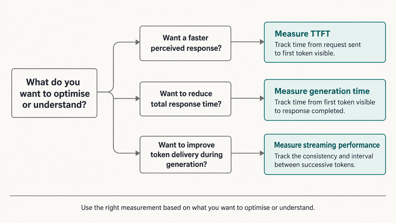
Published 30 October 2026. API prices checked 28–30 October 2026 on each provider’s official pricing page. Cost figures below are labelled as illustrative where they …
Indirect Prompt Injection

Gemini 4 Carbon Hit 0% on Indirect Prompt Injection. Is That Enough?

When Google announced Gemini 4 Carbon on 28 October, one line in the safety section stood out. Carbon scored 0.0% on Gray Swan’s Indirect Prompt …

AI Chip Leasing Export Controls and the Tencent Deal

AI Chip Leasing Export Controls

Tencent has reportedly agreed to pay about $7 billion over five years for access to roughly 100,000 advanced AI chips it is not permitted to buy. The chips sit in Oracle data centres in South-East Asia. They will stay there.

The Financial Times reported the arrangement on September 30. Neither company has confirmed it. If it is accurate, it describes something export-control law was not originally built to analyse: the hardware never moves toward the restricted destination, but the capability the hardware produces becomes available to a company inside it.

That is a genuinely difficult question, and most coverage has answered it too quickly in both directions. Calling it a loophole assumes the rules ignore remote access, which is not quite right. Calling it obviously lawful assumes physical location settles the analysis, which is also not right.

The useful question is narrower: what exactly is the export-control system regulating — the chip, or what the chip can do for whom?

Key takeaways
  • The FT reported on September 30 that Tencent signed a five-year lease worth about $7 billion for access to roughly 100,000 advanced AI chips in Oracle data centres in South-East Asia, with about 30% paid upfront. Neither company has confirmed it.
  • Under longstanding BIS practice, remote access to computing power is generally not treated as an export of the underlying chip. That is the basis of the gap argument, and it is only part of the picture.
  • BIS’s January 2026 rule conditions licences for China-destined advanced chips on KYC screening of remote users and, for IaaS providers, identification of remote end users in countries of concern. The rules already reach past the hardware.
  • End-use and end-user prohibitions under EAR Part 744 apply regardless of where hardware physically sits.
  • The contrast case is physical: DOJ alleges a California man routed more than $300 million in export-controlled GPU servers to China through Malaysia and Singapore. That conduct sits squarely within the existing framework. Offshore compute leasing is a different mechanism.
  • As compute becomes a financeable, leasable asset — NVIDIA’s $500 billion financing push treats chips as collateral — the distinction between owning hardware and buying its output becomes commercially central as well as legally awkward.
  • Nothing here is legal advice, and nothing in this article concludes that the reported arrangement is lawful or unlawful.

Quick Navigation


The Chip Stayed Put. The Compute Didn’t.

Seven arrangements get flattened into “getting chips,” and they are not legally equivalent. Separating them is the single most useful thing an article on this subject can do.

ArrangementWhat movesWho holds the hardware
Physical exportA controlled item crosses a borderThe recipient
Ownership transferTitle changes handsThe buyer, wherever it sits
Hardware leasePossession and use of physical serversThe lessee, physically
Compute leasingContractual access to capacityThe operator keeps the hardware
Cloud / GPU-as-a-serviceRemote consumption of cyclesThe provider
Offshore data-centre accessRemote use from another jurisdictionThe third-country operator
Diversion / transshipmentHardware routed to a prohibited destinationUltimately the prohibited end user
AI Chip Leasing Export Controls

The first three and the last involve physical items changing location or control. The middle three do not. Export-control law was built mainly around the first category and has been extended, through end-use and end-user rules, toward the others.

The important distinction is this: an export-control analysis asks what item went where, to whom, and for what use. A compute lease changes the answer to the first question without necessarily changing the answers to the other three.

What Export Controls Actually Control

The US framework for advanced AI chips runs through the Export Administration Regulations, administered by the Bureau of Industry and Security at the Commerce Department. Four mechanisms do most of the work.

  • Item-based controls. Advanced computing integrated circuits above performance thresholds are classified under specific ECCNs and require licences for certain destinations. This is the hardware layer.
  • Destination controls. Licence requirements and review policies vary by country, with China and Macau subject to the most restrictive treatment.
  • End-user controls. The Entity List and related restrictions attach to named parties regardless of where a transaction occurs. A listed party cannot receive controlled items anywhere.
  • End-use controls. EAR Part 744 prohibits certain uses — military, military-intelligence, WMD-related — and these prohibitions apply with knowledge, irrespective of geography.

Two further features matter for this story. The Foreign Direct Product Rule extends US jurisdiction to certain foreign-produced items made with US technology, which is how controls reach chips fabricated outside the United States. And the Data Center Validated End User framework, introduced in October 2024 and expanded in the January 2025 AI Diffusion Rule, created a route for approved operators to receive controlled chips for data centres abroad, with per-company and per-country computing-power limits. The Diffusion Rule itself was rescinded, but several of its structural ideas persist in current licence conditions.

In practical terms: the chip has to be licensed to get into the data centre in the first place. Whatever happens afterwards, the hardware entered under US authority and conditions.

Where AI Chip Leasing Export Controls Get Complicated

Start with the point everyone cites, stated precisely: under longstanding BIS practice, providing remote access to computing power is generally not treated as an export of the chips themselves. The item does not move. No licence requirement attaches merely because a foreign user runs a job on a US-origin GPU located abroad.

That principle is real, it is not a drafting oversight, and it exists for a defensible reason. Treating remote access as an export would mean every cloud login from a foreign IP address became a licensable event, which would be unenforceable and would damage US cloud providers more than it would constrain anyone else.

Now the complications, each of which is documented.

  • Licence conditions already reach remote users. BIS’s final rule effective January 15, 2026 moved China and Macau-destined advanced computing exports to case-by-case review, conditioned on certifications. Those conditions include rigorous KYC procedures by the ultimate consignee to screen and prevent unauthorized remote access by prohibited end users, and where the consignee provides IaaS, identification of intended remote end users in countries of concern plus controls against illicit access. Law-firm analysis of the rule described it as a notable departure from the practice that remote access alone is not an export.
  • End-user prohibitions do not care about geography. If a party is on the Entity List, supplying it with controlled items is prohibited wherever that happens. Whether a compute lease constitutes supplying an item is exactly the hard question, but the prohibition is not switched off by the hardware staying put.
  • End-use prohibitions travel. Military-intelligence and WMD-related end uses trigger requirements with knowledge, regardless of location. BIS has warned that exports to foreign cloud providers can trigger licence requirements under catch-all controls where there is knowledge of a prohibited end use.
  • Model weights are separately controlled. The January 2025 framework brought the most advanced model weights into scope, and IaaS commitments in current licence conditions address the transfer of weights trained on controlled chips. Compute leases produce weights; that output has its own treatment.

So the honest formulation is not “export controls do not cover this.” It is that hardware controls and compute access operate on different regulatory dimensions. The hardware layer is licensed, located and countable. The access layer is contractual, remote and attributed through the operator’s own diligence. The rules reach into the second layer mainly through conditions imposed at the first.

The South-East Asia Model

What the FT reported, stripped to verified elements: a five-year agreement signed this year, roughly $7 billion in value, about 30% paid upfront, access to approximately 100,000 advanced AI chips across multiple Oracle data centres in South-East Asia, for use in developing Tencent’s AI models and agentic tools.

What has not been reported: the chip generations, the host countries, the ownership structure, the contractual form, or any licensing position taken by either party. Those unknowns matter, because each would change an export-control analysis. The article’s analysis is therefore about the model, not about this transaction’s legality.

The pattern is not new. Reporting has described Tencent accessing NVIDIA Blackwell capacity through a data centre near Osaka in December 2025, and ByteDance’s Singapore subsidiary accessing B200 GPUs through a UK provider’s facility in Norway. What is new is scale: a nine-figure chip count and a ten-figure contract with a major US cloud provider.

Why this structure is commercially attractive is not mysterious:

  • Speed. Capacity exists now. Building domestic alternatives takes years.
  • Capability. The chips are generations ahead of what is available inside China.
  • Financial form. An operating expense with 30% upfront, rather than a capital purchase requiring import approval.
  • Regulatory posture. It avoids the question of importing hardware entirely, on both the US and Chinese sides.

For Oracle, the attraction is equally plain: a five-year anchor tenant with a large upfront payment underwriting South-East Asian capacity.

The analytical point: this is what happens when the regulated object is scarce but the service it produces is fungible and remotely deliverable. Demand routes to wherever the capability can be lawfully consumed.

A Server in Malaysia Is Not a GPU in China

On October 1, 2026, the Justice Department announced the arrest of Greg Lui, 38, also known as Yiu Kong Lui, of San Gabriel, California, owner of Earthmade Computer. A grand jury returned a three-count indictment on September 29 charging conspiracy to violate the Export Control Reform Act and the EAR, outbound smuggling, and conspiracy to commit money laundering.

Prosecutors allege that between 2023 and 2024 Lui and co-conspirators bought export-controlled servers containing US-made GPUs from American suppliers and shipped them through freight forwarders to countries including Malaysia and Singapore, using false paperwork, while knowing the true end users were in China. The release describes one January 2024 shipment of 27 servers sent from Los Angeles to Kuala Lumpur, allegedly forwarded to a buyer in China.

These are allegations. Lui is presumed innocent unless and until proven guilty.

Place that next to a compute lease and the difference is structural rather than moral:

Alleged diversionOffshore compute access
What movesPhysical serversNetwork traffic
Where the hardware ends upAllegedly ChinaStays in the third country
Evidence trailShipping records, invoices, customs filings, emailsContracts, access logs, billing records
Who investigatesBIS Export Enforcement, DOJ, customsPrimarily the operator’s own compliance function
Legal theoryEstablished: unlicensed export, smugglingDepends on end user, end use and licence conditions

The first column describes conduct the existing system was designed to catch, and it caught it. Physical goods generate documents, and documents generate cases.

The second column produces almost none of that. There is no shipment, no customs entry, no freight forwarder. There is a commercial contract between a cloud provider and a customer, and the record of who ran what is held by the provider.

For an enforcement agency, this means the investigative starting point moves from the border to the data centre’s customer list. That is a different kind of work, requiring different access, and it is the practical sense in which something has changed — not that the law is silent, but that the evidence lives somewhere else and belongs to someone else.

The Law Was Written Around Hardware. AI Is Becoming a Service.

Export controls assume a world of discrete items with owners and locations. That assumption is weakening on the commercial side faster than on the legal side.

NVIDIA announced partnerships in August 2026 with Apollo, BlackRock, Blackstone, Brookfield, Goldman Sachs and KKR around financing platforms intended to mobilise more than $500 billion for AI infrastructure. Jensen Huang told CNBC that this is the first time technology chips have become an investable asset class, arguing that because the hardware is broadly adopted and transferable, lenders can underwrite compute as a revenue-generating asset. NVIDIA has indicated it may provide residual-value support of up to 25% on some projects.

The structure is ordinary equipment finance applied to accelerators: a financing vehicle buys the hardware, an operator leases it, customer contracts produce the cash flows, and the debt is secured against both. CoreWeave’s $8.5 billion GPU-backed facility earlier this year is the proof of concept.

Reuters reported in early October that bankers and asset managers want more guarantees before treating these chips as long-term collateral, with one portfolio manager noting that Wall Street is more conservative than NVIDIA’s decade-long revenue claim implies. That scepticism is about residual value, which is the same obsolescence problem we worked through in our analysis of AI accelerator depreciation.

Here is why this belongs in an export-control article. The financing model deliberately separates three things that used to travel together: who owns the chip, who operates it, and who consumes its output. A financing vehicle may own it, an operator may run it, and a customer in a third jurisdiction may use it. Every one of those can be a different legal person in a different country.

Export-control analysis has to pick one of those relationships to attach to. Historically it attached to ownership and location. The commercial structure is moving the economic substance toward consumption.

China’s Two Paths to Compute

Chinese AI developers have two routes to frontier-scale compute, and they operate on completely different timescales.

  1. Domestic silicon is the sovereign answer and the slow one. Alibaba’s T-Head unveiled its Zhenwu V900 accelerator in September, claiming clusters scaling to 500,000 cards, and Huawei continues to iterate its Ascend line. The constraint is not design talent. It is manufacturing, advanced packaging and high-bandwidth memory supply, all of which are themselves export-controlled or capacity-limited — the chain we examined in our piece on the memory wall behind a 500,000-card cluster.
  2. Offshore leased compute is the fast answer. It delivers current-generation capability immediately, with no fabrication, no packaging and no domestic approval process for imported hardware.

The two are complements rather than alternatives, and the comparison should not be overstated. Offshore capacity cannot serve latency-sensitive domestic products well, cannot be used for workloads with data-residency constraints, and leaves the customer dependent on a foreign provider and a foreign regulator. It buys training capability, not infrastructure sovereignty.

The analytical read: domestic silicon addresses the long-run strategic problem; offshore leasing addresses the immediate capability gap. A company pursuing both is behaving rationally, and the existence of the second does not reduce the urgency of the first.

The Enforcement Problem

Even where rules clearly apply, applying them to compute access is harder than applying them to cargo. Five reasons, none of which is a legal gap as such.

  1. Attribution. A shipment has a consignee. A compute workload has an account, which may belong to a subsidiary, a joint venture or a reseller. Determining who is actually running a job is a diligence exercise, not a customs check.
  2. Beneficial ownership. End-user rules attach to parties, and corporate structures can obscure which party a customer ultimately belongs to. This is why current licence conditions push KYC obligations onto the consignee — the operator is better placed than the regulator to know its own customers.
  3. Jurisdiction. The chips are US-origin and subject to the EAR. The data centre sits in a third country under that country’s law. The customer is in a fourth. US authority reaches the hardware; reaching the commercial relationship around it depends on the conditions attached when the hardware was licensed.
  4. Visibility. Access records belong to the operator. There is no equivalent of a customs declaration that a government sees by default.
  5. Fungibility. Compute is not a widget. The same cluster serves many customers and many workloads, which makes a per-job determination about end use far harder than a per-shipment one.

To be explicit about what this article will not do: none of the above is a description of how to structure an arrangement to avoid controls, and nothing here recommends jurisdictions, structures or practices for that purpose. The point is the opposite — these are the features that make compliance and oversight demanding for everyone operating legitimately.

The Bear Case: Why the Gap May Be Smaller Than It Looks

The loophole framing assumes a static rulebook. Several things cut against it.

  • The hardware was licensed under conditions. Those chips reached a South-East Asian data centre through the US export-control system. Conditions imposed at that point — KYC, remote-user identification, IaaS commitments, prohibitions on serving restricted end users — travel with them.
  • BIS has already moved. The January 2026 rule conditions China-destined licences on exactly the remote-access questions this article is about. Analysts described it as a departure from the position that remote access alone is not an export, and as a possible precursor to broader reconsideration.
  • Legislation is pending. The Remote Access Security Act, if enacted, would make cloud access to controlled computing explicitly subject to controls. It has not passed, and the article does not assume it will.
  • Cloud providers have strong incentives. A major US provider risks its licences, its reputation and potential enforcement exposure. Compliance functions at that level are not nominal.
  • Diligence guidance already exists. BIS has published due-diligence expectations for parties dealing with advanced computing ICs, including evaluating data centres and IaaS providers, which assumes the compute-service layer is within the regulatory field of view.
  • The policy scenario worth watching: if policymakers conclude that access to compute is strategically equivalent to possession of chips, the regulatory object changes from an item to a service. That would mean licensing compute capacity by customer and country, mandatory KYC for AI-scale workloads, reporting of large training runs, and possibly technical attestation of what runs where. Each is conceivable. Each would land hardest on compliant US providers, which is the central argument against doing it, and the reason it remains a scenario rather than a forecast.

What AI Infrastructure Buyers Should Watch

Different parties face different exposure here, and the practical implications diverge.

  • Cloud and data-centre operators carry the heaviest load. Licence conditions push KYC and remote-user identification onto the consignee, which means the operator is the compliance perimeter. Worth confirming: what your licences actually require, whether customer screening extends to affiliates and ultimate parents, how remote-user records are retained, and whether your contracts let you terminate access on a compliance determination.
  • Enterprises buying compute should know where their capacity physically sits and under what authorisation. A capacity contract with an offshore provider carries counterparty risk that is regulatory as well as commercial. If rules tighten, access can be curtailed by someone else’s licence condition.
  • Investors in AI infrastructure should treat regulatory exposure as part of the asset analysis. A facility whose economics depend on a single large customer from a sensitive jurisdiction has a concentration risk that no residual-value guarantee covers.
  • Chip financiers face a version of the same problem. If compute access becomes licensable, the cash flows securing a GPU-backed facility become dependent on continued regulatory permission for specific customers.

The indicators worth tracking over the next year:

  • Whether BIS issues guidance or rulemaking addressing remote access directly
  • Whether the Remote Access Security Act or similar legislation advances
  • Enforcement actions involving cloud access rather than physical diversion
  • New licence conditions attached to data-centre exports
  • Whether allied jurisdictions hosting this capacity adopt parallel requirements
  • Public confirmations or denials from Oracle or Tencent
  • The pace of Chinese domestic accelerator deployment, which determines how long offshore demand persists

The Two Objects

The physical chip and the computing capability it produces are becoming two different economic objects, and the regulatory system currently has a mature apparatus for one of them.

For the chip, there are classifications, licences, thresholds, destination rules, customs records and prosecutions. The Lui indictment shows that machinery working as intended: documents, shipments, a paper trail, charges.

For the capability, there is a growing set of conditions attached to the hardware’s export and a heavy reliance on operators to police their own customer lists. That is not nothing. It is a different kind of control, enforced at a different point, with evidence held by private parties.

Whether that constitutes a gap depends on what you think controls are for. If the objective is preventing controlled hardware from reaching restricted destinations, the current system is working and the Tencent arrangement does not defeat it. If the objective is preventing restricted parties from obtaining frontier AI capability, hardware location is an increasingly indirect proxy for the thing being controlled.

That is the question policymakers have not yet answered out loud, and every structure described in this article is a bet on which answer arrives first.

FAQ

This section is informational analysis, not legal advice. Anyone with a live transaction should take export-control counsel.

What are AI chip leasing export controls?

The term describes how US export rules apply when a customer leases access to advanced AI chips rather than buying them. The chips themselves are controlled under the Export Administration Regulations and require licences for certain destinations and end users. Leasing arrangements raise a separate question: whether providing remote access to those chips’ computing power is itself a controlled activity.

Can companies legally lease AI compute from another country?

Generally yes, subject to the applicable rules. Remote access to computing power is not ordinarily treated as an export of the underlying chip under longstanding BIS practice. That does not make any particular arrangement lawful: end-user restrictions, end-use prohibitions and conditions attached to the chips’ original export licences all continue to apply.

Do US export controls apply to offshore GPU cloud services?

In several ways. The chips must be lawfully exported to the data centre. Licence conditions issued since January 2026 for China-destined advanced chips require the consignee to apply KYC screening to prevent unauthorized remote access and, where it provides IaaS, to identify remote end users in countries of concern. Prohibitions on supplying listed parties or prohibited end uses apply regardless of location.

Is renting GPU compute the same as importing AI chips?

No. Importing involves a physical item crossing a border with an identifiable consignee and customs record. Renting compute involves a contractual right to run workloads on hardware that stays where it is. The export-control analysis differs because the regulated item does not move, though end-user and end-use rules still apply.

Why are companies using offshore AI compute?

Speed and capability. Capacity exists now, the hardware is generations ahead of what is available inside China, and the arrangement is an operating expense rather than a capital import requiring approval on both sides.

Can China access advanced AI chips through overseas data centres?

Chinese companies have accessed overseas compute capacity, as reported in the Oracle-Tencent case and earlier arrangements in Japan and Norway. Whether a specific arrangement complies with US controls depends on the end user, the end use, and the conditions attached to the chips’ export. No public determination has been made about the reported Oracle arrangement.

What is the difference between the DOJ smuggling case and offshore compute leasing?

In the DOJ case, prosecutors allege physical servers were routed to China through third countries using false paperwork. Those are allegations and the defendant is presumed innocent. In offshore leasing, the hardware stays in the third country and only network traffic crosses borders. The first is a classic export-control violation theory; the second turns on different questions.

Will export controls eventually cover AI compute access?

Possibly. The Remote Access Security Act would make cloud access to controlled computing explicitly subject to controls, but it has not been enacted. Current licence conditions already impose KYC and IaaS obligations that reach remote users indirectly. Whether that extends into direct regulation of compute access is a policy choice that has not yet been made.


Keep reading

Types of AI Models

Types of AI Models in 2026: A Field Guide From LLMs to World Models

Model details checked against official announcements, model cards and documentation on 1 November 2026. Line up four AI models that were current at the end …
AI Coding Agent

AI Coding Agents Are Getting Expensive. Who’s Paying for the Tokens?

Pricing checked on official vendor pages on 1 November 2026. All USD. Cost scenarios are illustrative and labelled as such. On 28 October, TechCrunch published …
generative AI architecture

Generative AI Architecture: The 7 Layers That Are Hard to Undo
Published 30 October 2026. API prices checked 28–30 October 2026 on each provider’s official pricing page. Cost figures below are labelled as illustrative where they …
Indirect Prompt Injection

Gemini 4 Carbon Hit 0% on Indirect Prompt Injection. Is That Enough?

When Google announced Gemini 4 Carbon on 28 October, one line in the safety section stood out. Carbon scored 0.0% on Gray Swan’s Indirect Prompt …

HBM Pricing 2027: What Locked Contracts Fix in Your Budget

HBM pricing 2027

If you are building an AI infrastructure budget for 2027, one line item just moved from the forecasting column to the contracts column. Micron told investors on September 30 that it has completed agreements covering the vast majority of its calendar 2027 HBM bit supply, at significant year-over-year price increases.

Read that twice, because it says two different things. The quantity question for a large share of next year’s high-bandwidth memory is settled. So is the price, and the price went up.

For anyone modelling accelerator costs, that is a strange kind of good news. Uncertainty is expensive — it forces contingency, it delays commitments, it makes the finance conversation harder. Removing it is worth something. But the uncertainty is being removed at a level above where most 2026 budgets assumed it would land, and the memory line in an AI server bill of materials is large enough that the difference shows up in cost per token.

This is not a Micron earnings recap. The question worth working through is narrower: with most of 2027’s HBM already spoken for at known prices, what can an infrastructure buyer now treat as fixed, and what is still genuinely open?

Key takeaways
  • Micron CEO Sanjay Mehrotra said the company has completed agreements for the vast majority of its calendar 2027 HBM bit supply, with significant year-over-year price increases that are narrowing the gross-margin gap between HBM and conventional DRAM.
  • The fiscal Q4 numbers behind that statement: revenue of $54.2 billion, gross margin of 87.0%, non-GAAP EPS of $33.42, and full-year revenue of $133.2 billion, up 256%.
  • Fiscal Q4 DRAM revenue rose 27% sequentially to $39.8 billion, but bit shipments grew only in the mid-single digits while average selling prices rose in the high teens. Revenue growth is coming from price, not volume.
  • Contracted pricing reduces budget variance without reducing cost. The planning problem changes shape rather than going away.
  • Micron is working with NVIDIA on what it calls the industry’s first custom HBM4E implementation, NVHBM, for next-generation GPUs and NVLink Fusion platforms — a development that cuts against the assumption that HBM is becoming more substitutable.
  • The bear case is real but mostly concerns 2028 and beyond: additional qualified supply, yield improvements and capacity additions take time to reach volume.

Quick Navigation


The Number Infrastructure Buyers Should Actually Read

The headline numbers from Micron’s fiscal fourth quarter are striking, and almost none of them change how you budget.

MetricFiscal Q4 2026Context
Revenue$54.2bnUp 31% sequentially, up 379% year over year
Gross margin87.0%Up 210 basis points sequentially
Non-GAAP EPS$33.42Up 33% sequentially
DRAM revenue$39.8bn73% of company revenue, up 27% sequentially
Full-year revenue$133.2bnUp 256%, with DRAM alone above $100bn

Those are results. The sentence that matters for planning is a forward one, from Mehrotra’s prepared remarks: Micron has completed agreements for the vast majority of its calendar 2027 HBM bit supply, with significant price increases year over year, narrowing the gross-margin gap with conventional DRAM.

On the call he put it more bluntly, noting that 2026 HBM prices were negotiated with customers the previous year, that a large part of the 2027 volume is already sold out, and that 2027 prices are much higher than 2026’s.

Four different things get confused in coverage of this, and separating them is the whole basis for using the information:

  • Reported financial results describe a quarter that closed in early September. They are history.
  • Contracted pricing is what Micron and its customers have agreed for future delivery. This is the forward-looking part, and it is what the 2027 statement refers to.
  • Current market pricing is where memory trades today, which can move independently of either.
  • Future supply conditions are what capacity, yield and qualification produce over the next two years.

The September results do not tell you what HBM costs today. The contracting statement tells you something more useful: that a large share of next year’s supply has a price attached already, and that the price was set in a market where suppliers had the leverage.

Why HBM Pricing 2027 Is Not a Commodity Memory Question

High-bandwidth memory is DRAM stacked vertically, connected by through-silicon vias, and packaged next to the processor on the same substrate. The point is bandwidth: an accelerator generating tokens reads weights and cache continuously, and the memory path, not the arithmetic, usually sets the pace.

That physical arrangement is why HBM does not price like the DRAM in a laptop.

  • It consumes disproportionate wafer capacity. Stacked dies with TSV structures use substantially more silicon per usable gigabyte than standard DRAM, so every HBM bit displaces several conventional ones. Industry analysts have consistently described HBM wafer intensity as multiples of DDR5, which is why the AI build-out has pulled supply away from commodity memory.
  • It is packaging-constrained, not just fab-constrained. HBM needs advanced packaging to attach to the accelerator. Capacity at that stage is a separate bottleneck with its own lead times.
  • Yields are harder. Stacking twelve or sixteen dies and having the result work is a different manufacturing problem from producing one good die.
  • Supply is qualified, not fungible. An accelerator vendor validates a specific supplier’s specific product for a specific platform. You cannot substitute an unqualified part because the price is better. Qualification has historically taken quarters, and missing a window has cost suppliers entire product cycles.
  • It sells on long-term agreements. Because of all of the above, HBM is contracted ahead rather than bought on spot. That is the mechanism behind the 2027 statement, and it is also why HBM prices are stickier in both directions than commodity DRAM.

The practical implication: HBM behaves less like a commodity input and more like a negotiated, capacity-reserved component — closer to how you would buy fab capacity than how you would buy RAM. We worked through the cost side of this in our breakdown of AI memory costs.

Revenue Growth Is Not Capacity Growth

The DRAM figures are where the pricing environment becomes visible, and they are worth reading carefully rather than celebrating.

Fiscal Q4 DRAM revenue was $39.8 billion, up 27% sequentially. Over the same period, bit shipments rose only in the mid-single-digit percentage range while average selling prices rose in the high teens.

That decomposition is the story. Roughly a fifth of the sequential revenue growth came from selling more bits; the rest came from charging more for them.

  • For a supplier, that is pricing power — demand exceeding available supply, with customers accepting higher prices rather than going without.
  • For a buyer, it means the thing you are budgeting for is not getting more plentiful. Capacity grew slowly. Price did the work.

Two cautions about how far to push this. These are sequential, quarter-over-quarter figures for DRAM overall, not HBM specifically, and Micron does not break out HBM revenue separately. And one quarter’s price-volume split does not establish a trend — though Micron’s own guidance for the following quarter, revenue of about $61.5 billion with gross margin near 86%, suggests the company does not expect the environment to normalise immediately.

The useful inference for planning: if supply were expanding quickly, suppliers would be competing on volume. They are not. That is consistent with the capacity picture the rest of the industry has described, and it is the context in which 2027 contracts were negotiated.

What the 2027 Contracts Actually Lock In

The important distinction is between price uncertainty and high but contracted pricing. They feel similar on a spreadsheet and behave completely differently in a planning cycle.

Uncertainty costs you optionality. You hold contingency, you defer commitments, you build scenarios, and you argue with finance about a range rather than a number. Contracted pricing costs you money — but it costs a known amount, on a known schedule, which is a materially easier object to plan around.

HBM pricing 2027

What is now more knowable:

  • A large share of 2027 HBM volume has a buyer and a price
  • Micron’s exposure to spot volatility for that volume is reduced, and so is its customers’
  • The direction of travel is established: 2027 pricing is above 2026 pricing, by the supplier’s own description
  • The margin structure is converging, with HBM’s gross-margin gap to conventional DRAM narrowing

What this does not tell you:

  • The actual price. “Significant increases” is a characterisation, not a number, and the contracts are private.
  • Which customers hold the allocation. “Sold out” says nothing about who holds it.
  • What is left. “Vast majority” implies a remainder, unquantified.
  • What the other two suppliers agreed. SK hynix and Samsung negotiate separately.

For an infrastructure buyer the implication splits by position. If you have a long-term agreement, your 2027 memory cost is largely a known quantity and the planning problem is a budget problem. If you are buying through an OEM or a cloud provider, your exposure is to their contracts, with a margin on top. If you are hoping to buy into the remainder, you are competing for the leftover in a market the supplier describes as largely committed.

What HBM Pricing 2027 Still Leaves Open

Contracted does not mean settled. Four variables stay live.

  1. Allocation versus commitment. A contract for bits is not a guarantee of delivery schedule or configuration. Capacity per accelerator and stack height can change what a given bit commitment actually equips.
  2. Generation mix. HBM3E, HBM4 and HBM4E coexist across platforms. Which generation your accelerators require affects both price and availability, and the generations are not interchangeable.
  3. Qualification outcomes. Supplier share on a given platform depends on qualification, which continues to move. Third-party reports on HBM4 allocations have conflicted repeatedly through 2026 — some placing Micron at roughly a fifth of NVIDIA’s HBM4 allocation, others describing it as excluded from initial Rubin builds. These are supply-chain research claims, not company disclosures, and should be treated as contested.
  4. Everything downstream of the chip. Packaging capacity, server assembly, power availability and data-centre readiness all sit between a contracted bit and a running accelerator. A fixed memory price does not fix a delivery date.

How HBM Pricing 2027 Lands in AI Server Economics

Memory does not determine accelerator economics on its own. It is one input among several, and the honest version of this section is about where in the chain it shows up.

  • In the bill of materials. HBM is one of the largest single cost components in an AI accelerator module, alongside the logic die and the packaging. A higher contracted memory price raises the module cost, which raises the server cost, which raises what a rack costs to stand up. None of the other components get cheaper to compensate.
  • In depreciation. A more expensive asset depreciated over the same period produces a higher capital charge per hour. That flows into every internal rate and every build-versus-rent comparison, as we worked through in our piece on accelerator depreciation.
  • In cost per unit of useful work. This is where it either hurts or does not. A higher hourly cost divided by more useful output per hour can net out flat. Memory capacity and bandwidth are also what let a model fit, batch larger and serve longer contexts — so the expensive component is the one buying the throughput. Whether the trade is favourable depends almost entirely on utilisation, which we examined in our analysis of accelerator utilisation.
  • In cloud pricing. Providers facing higher input costs either absorb them, pass them through, or change instance mix. All three have happened in previous cycles. For anyone renting rather than building, the exposure is indirect and lagged, but it is not absent.

The analytical point worth holding onto: a contracted higher memory price makes the capital side of the equation more predictable and more expensive, while leaving the output side entirely in the operator’s hands. Two organisations buying identical hardware at identical contracted prices can still end up with cost per token that differs by multiples, because utilisation and serving efficiency are not contracted by anyone.

The Bear Case Against the HBM Pricing 2027 Thesis

Every memory cycle in history has ended with oversupply. Assuming this one is different is how people lost money in 2018. Here is what could weaken the pricing picture, with an honest view of the timing.

  • More qualified suppliers. Three vendors compete in HBM, and their relative positions keep moving. Samsung’s qualification progress at NVIDIA has been the single most-watched variable in this market for two years, and a stronger Samsung position would give buyers a third credible source at the top of the stack. Reports on HBM4 allocation have conflicted enough through 2026 that nobody outside the negotiations should be confident about share.
  • Capacity additions. Every supplier is investing heavily. HBM capacity added in 2026 arrives through 2027 and 2028.
  • Yield improvements. A yield gain is effective capacity at no additional capital cost, and stacking yields improve as processes mature. This is the quietest and often the fastest source of supply growth.
  • HBM4 and HBM4E transitions. Generational transitions redistribute share. A supplier that executes well on a new generation can gain allocation quickly; one that stumbles loses a cycle.
  • Demand normalisation. The demand side assumes continued aggressive AI infrastructure spending. Hyperscaler capex plans are revised more often than they are announced.
  • Alternative architectures. Approaches that reduce memory pressure per unit of output — better quantisation, more efficient attention, memory-efficient serving — reduce how much HBM a given workload requires.

Now the counterargument, which is the more interesting half.

Micron’s collaboration with NVIDIA on NVHBM, described as the industry’s first custom HBM4E implementation for next-generation GPUs and NVLink Fusion platforms, points the other way. Custom memory designed for a specific platform is harder to second-source than a standard part. If the industry moves toward platform-specific HBM, the thing that normally ends a memory cycle — commoditisation and substitution — gets harder, not easier. Switching costs rise, qualification becomes more bespoke, and pricing power persists longer than the capacity numbers alone would suggest.

There is also the structural change in how this market transacts. Long-term agreements covering a large share of volume dampen the spot-price dynamics that historically turned a supply increase into a price collapse within a quarter. Contracts do not prevent a downturn; they delay and smooth it.

Which force wins is not knowable from here, and anyone claiming otherwise is guessing. What can be said with reasonable confidence is about timing: capacity, yield and qualification all operate on multi-quarter cycles, and 2027’s supply is already largely committed. A meaningful loosening is a 2028 question.

What to Change in a 2027 Budget

The practical shift is from modelling a range to negotiating a number, and from arguing about memory cost to arguing about memory-cost-per-unit-of-output.

What can now be budgeted with more confidence:

ItemWhy it firmed up
Direction of HBM pricing into 2027The supplier has stated significant year-over-year increases
Availability of contracted volumeMost of Micron’s 2027 bits are committed, which also means allocated
Supplier margin postureThe HBM-to-DRAM margin gap is narrowing, so discounting is unlikely
Memory as a share of accelerator costRising, not falling, for the next cycle

What stays uncertain, and should keep a contingency line:

ItemWhy it is still open
Your actual unit priceContracts are private and vary by customer and volume
Generation and configurationCapacity per accelerator and stack height affect total cost
Supplier share on your platformQualification outcomes continue to move
Delivery timingPackaging, assembly and data-centre readiness are separate constraints
2028 and beyondCapacity additions and yield gains land after the contracted window

Three budgeting moves follow from that split.

  1. Model memory as a contracted input, not a market input. If you buy at scale, that means getting a number into the agreement rather than carrying a range. If you buy through an OEM or cloud, it means asking what their exposure is and when their agreements renew.
  2. Stop assuming memory cost declines. The decades-long reflex that memory gets cheaper per bit does not apply to a supply-constrained component inside a capacity-limited manufacturing chain. Budgets built on an assumed annual decline are the ones that break.
  3. Shift the optimisation target. If the input price is fixed and rising, the remaining lever is output per unit of hardware. Utilisation, batching efficiency and serving architecture now carry more of the cost-reduction burden than procurement does.

A Procurement Checklist

Twelve questions worth having answers to before a 2027 plan is signed off.

  1. What is our contracted HBM price, and through what date?
  2. What volume is committed, and what are the penalties on both sides for missing it?
  3. Which HBM generation do our target accelerators require, and is that supply separately contracted?
  4. How much memory capacity per accelerator do our workloads actually need?
  5. Which suppliers are qualified on our platform, and what happens if one slips?
  6. What share of our accelerator BOM is memory, at contracted prices?
  7. Is packaging capacity a constraint on our delivery schedule, separately from chip supply?
  8. What depreciation period are we applying, and does it match how long the hardware stays competitive?
  9. What utilisation are we assuming, and what does cost per token look like at 50% of it?
  10. What are our power and cooling constraints, and do they bind before memory does?
  11. If we rent rather than buy, when do our provider’s input contracts renew?
  12. What is our exposure in 2028, when the contracted window closes?

Question 9 is the one that decides whether the higher contracted price actually hurts. A memory cost increase absorbed by better utilisation is an accounting event. The same increase on an under-utilised fleet is a budget problem.

FAQ

What will HBM pricing 2027 look like?

Higher than 2026, by the supplier’s own account. Micron said on September 30, 2026 that it had completed agreements for the vast majority of its calendar 2027 HBM bit supply with significant year-over-year price increases. The actual contract prices are private, and no credible public source provides a specific 2027 price, so treat any precise figure you see with suspicion.

Why is HBM so expensive?

Because it consumes far more wafer per usable gigabyte than standard DRAM, requires stacking many dies with through-silicon vias at yields that are harder to achieve, and depends on advanced packaging capacity that is itself constrained. It is also qualified per platform rather than interchangeable, which limits competitive pressure.

Why are HBM prices rising?

Demand from AI accelerators is growing faster than qualified supply. Micron’s fiscal Q4 figures illustrate the environment: DRAM revenue rose 27% sequentially while bit shipments grew only mid-single digits and prices rose in the high teens.

How do HBM contracts affect AI server costs?

They convert a variable input into a fixed one at a higher level. Memory is among the largest components in an accelerator’s bill of materials, so a contracted increase raises server cost, capital charge per hour and the floor under cost per token — predictably rather than unpredictably.

Who supplies HBM for AI accelerators?

Three companies: SK hynix, Samsung and Micron. Share depends on qualification at accelerator vendors, and it shifts by generation. Public reporting on HBM4 allocations has been inconsistent through 2026, so supplier share should be treated as contested rather than settled.

Can HBM prices fall in 2027?

For supply already under contract, the price is agreed and falling spot prices would not change it. Broader softening would need capacity additions, yield improvements or demand normalisation to arrive at volume — and those operate on multi-quarter cycles, which makes 2028 the more plausible window.

How does HBM affect GPU economics?

It is one input among several, and it works both ways. More memory capacity and bandwidth cost more and also let a model fit on fewer devices, run larger batches and serve longer contexts. Whether the higher price hurts depends mostly on utilisation.

What should AI infrastructure buyers budget for HBM?

Use your own contracted price if you have one, or ask your OEM or cloud provider about theirs. Do not budget an annual per-bit price decline for this component, and keep a contingency line for generation, configuration and delivery timing, which remain open even where price does not.


Keep reading

Types of AI Models

Types of AI Models in 2026: A Field Guide From LLMs to World Models

Model details checked against official announcements, model cards and documentation on 1 November 2026. Line up four AI models that were current at the end …
AI Coding Agent

AI Coding Agents Are Getting Expensive. Who’s Paying for the Tokens?

Pricing checked on official vendor pages on 1 November 2026. All USD. Cost scenarios are illustrative and labelled as such. On 28 October, TechCrunch published …
generative AI architecture

Generative AI Architecture: The 7 Layers That Are Hard to Undo
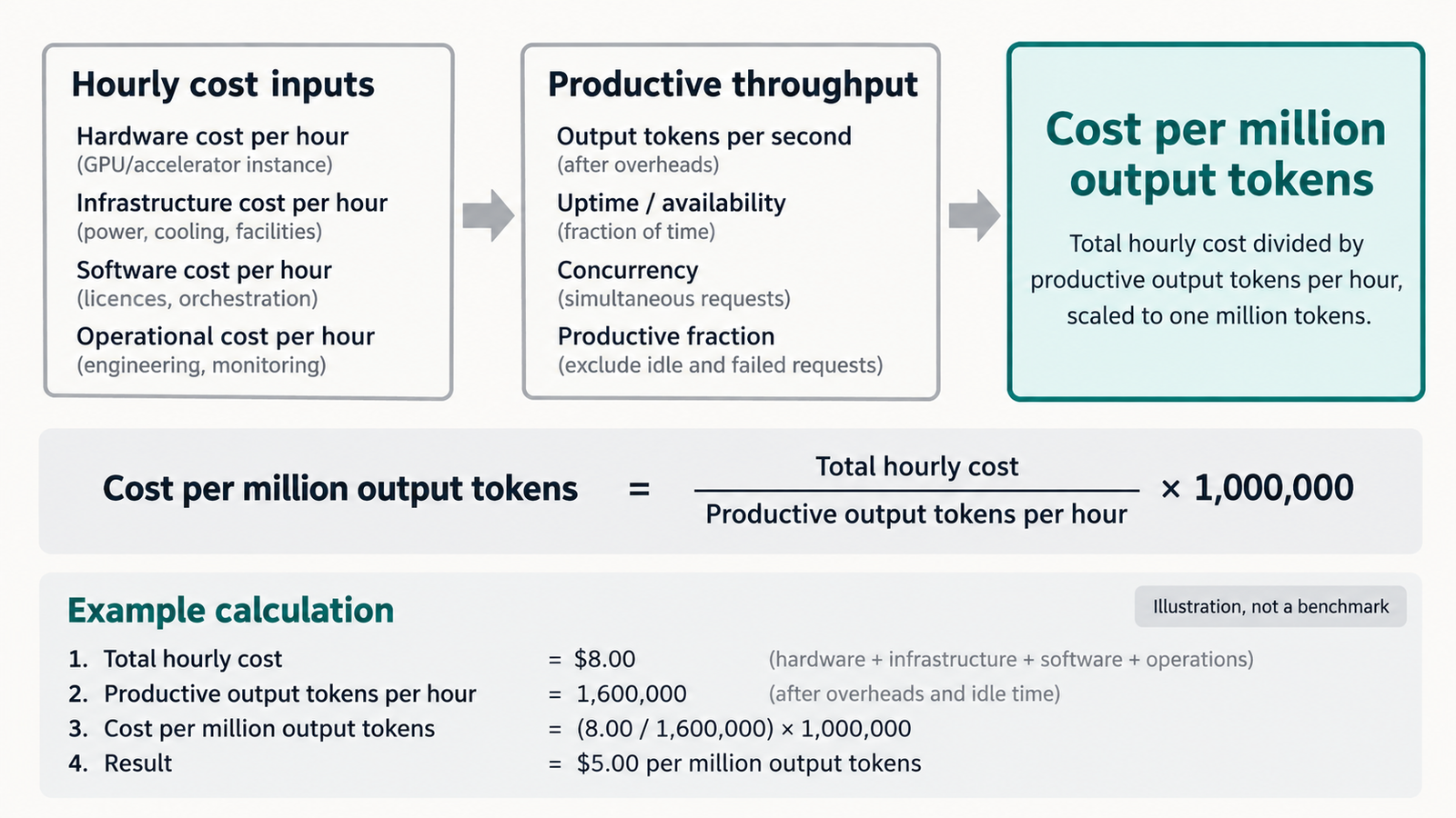
Published 30 October 2026. API prices checked 28–30 October 2026 on each provider’s official pricing page. Cost figures below are labelled as illustrative where they …
Indirect Prompt Injection

Gemini 4 Carbon Hit 0% on Indirect Prompt Injection. Is That Enough?

When Google announced Gemini 4 Carbon on 28 October, one line in the safety section stood out. Carbon scored 0.0% on Gray Swan’s Indirect Prompt …

AI Accelerator Depreciation: The Assumption Nobody Audits

AI accelerator depreciation

An A100 with 80GB of HBM2e still computes exactly as well in 2026 as it did when it was installed. Nothing has degraded. It passes every diagnostic.

It is also increasingly hard to justify running, and the reason has almost nothing to do with its arithmetic throughput. A model that fits comfortably in 141GB on an H200 must be sharded across two A100s, halving effective utilisation and doubling the interconnect traffic. A context window that one newer accelerator holds in its KV cache does not fit at all.

The hardware works. The workload moved.

That gap — between an accelerator that functions and one that earns — is the subject of this article, and it sits directly on top of an accounting assumption that carries tens of billions of dollars of reported profit across the industry. AI accelerator depreciation is the allocation of an accelerator’s cost across its estimated useful life, and the estimate is exactly that: an estimate, chosen by management, disclosed in a sentence, and rarely examined against the physics of the workloads the hardware actually has to serve.

Key takeaways
  • AI accelerator depreciation is an accounting allocation, not a measurement of hardware lifespan. The disclosed figure is an estimate of economic benefit, and the hyperscalers apply it to “servers and network equipment” as a category rather than to accelerators specifically.
  • Four different lifetimes hide inside one number: physical, accounting, economic and competitive. They rarely coincide, and the shortest one determines when replacement actually happens.
  • The hyperscalers no longer agree. Microsoft and Alphabet moved servers to six years in 2022–23 and have held there; Amazon shortened a subset back to five effective January 2025, citing the pace of AI development; Meta extended to 5.5 years the same month.
  • Changing a four-year assumption to three raises annual depreciation on the same asset by roughly a third, which flows straight into cost per accelerator-hour and cost per token.
  • Memory capacity is the underexamined obsolescence driver. Accelerator HBM has gone from 40–80GB on A100 to 141GB on H200, 192GB on B200 and up to 288GB on B300-class parts, while models, context windows and KV caches grew to match.
  • An accelerator becomes economically obsolete when the workload outgrows its memory envelope, not when it stops computing. We call this obsolescence by memory footprint — an analytical framing, not an accounting term.

Quick Navigation


AI Accelerator Depreciation Starts With an Accounting Assumption

Depreciation spreads the cost of a long-lived asset across the periods that benefit from it. For an accelerator bought outright, the mechanics are simple:

Annual depreciation = (asset cost − salvage value) ÷ estimated useful life

The cost is known. Salvage value for accelerators is usually assumed to be small or zero. Useful life is the judgement call, and it is the only input management chooses.

That choice does three things at once. It sets reported operating income, because depreciation is an expense. It sets the capital recovery burden built into internal transfer pricing and cloud rate cards. And it signals to investors how long management believes the hardware will produce economic benefit.

One structural point deserves emphasis before any of the numbers below. None of the major operators discloses a useful life specifically for AI accelerators. They disclose useful lives for categories such as “servers and network equipment” or “technical infrastructure”, which bundle accelerators with CPUs, memory, storage, chassis and switches. Treating a disclosed six-year server life as a statement about GPU lifespan is an inference, not a reading of the filing.


AI Accelerator Depreciation Hides Four Different Lifetimes

The same physical accelerator has four expiry dates, and they are set by different forces.

LifetimeWhat ends itWho decides
PhysicalComponent failure — HBM faults, VRM degradation, thermal damagePhysics and operating conditions
AccountingThe end of the disclosed useful lifeManagement estimate, audited for reasonableness
EconomicThe point at which running it costs more than the value it producesPower prices, utilisation, alternatives
CompetitiveThe point at which it cannot serve the workload at acceptable throughput, latency or memoryModel architecture and customer requirements

Physical life is usually the longest. Well-cooled data-centre hardware runs for many years, and the secondary market for previous-generation accelerators exists precisely because they still work.

Accounting life sits in the middle by construction, since auditors want an estimate that reflects expected economic benefit rather than either extreme.

Economic life turns on operating cost against output. An older accelerator drawing 400W to produce a fraction of what a newer part produces at 700W can lose on performance per watt badly enough that electricity alone justifies replacement, before any capital consideration.

Competitive life is usually the shortest, and it is the one nobody discloses. It ends when the accelerator can no longer hold what the workload needs it to hold.

The practical consequence: a fleet can be fully depreciated and still valuable, or carry substantial book value while being commercially unusable for current workloads. Neither situation is visible from the depreciation schedule.


What Major Operators Disclose About AI Accelerator Depreciation

Between 2022 and 2024 the major operators moved in one direction. In January 2025 they stopped agreeing.

CompanyDisclosed changeStated scopeReported effect
Microsoft4 → 6 years, effective FY2023 (July 2022)Servers and network equipment~$3.7bn lower depreciation, ~$3.0bn higher net income in FY23
AlphabetServers 4 → 6 years; certain network equipment 5 → 6, effective January 2023Servers and certain network equipment~$3.9bn lower 2023 depreciation, ~$3.0bn higher net income
Amazon5 → 6 years, effective January 2024Servers~$3.2bn lower 2024 depreciation, ~$2.5bn higher net income
Amazon6 → 5 years, effective January 2025A subset of servers and networking equipmentRoughly $0.7bn lower operating income, with accelerated depreciation on early retirements
MetaMost assets → 5.5 years, effective January 2025Servers and network assets~$2.9bn lower 2025 depreciation, ~$2.6bn higher net income
OracleExtended to 5 years, 2023Servers and related equipmentDisclosed in that year’s filing

Four points about how to read that table.

  1. The direction reversed, once. Amazon is the only operator in the group to have shortened, and its stated reason is specific: the increased pace of technology development, particularly in artificial intelligence and machine learning. That is a company statement about AI hardware turnover, from the operator with the largest cloud footprint.
  2. The categories are not comparable. Microsoft’s disclosure covers servers and network equipment together as a range of two to six years. Alphabet separates servers from certain network equipment. Amazon’s January 2025 change applies to a subset it does not size. Lining these up in one column is convenient and slightly misleading, which is why the scope column is there.
  3. Sources disagree on some figures. Alphabet’s 2023 effect appears in coverage as both a ~$3.9bn actual reduction and a ~$3.4bn estimate made at the time of the change. Those are different things — an estimate disclosed in the 2022 10-K versus the outcome reported later — and the difference is a good illustration of why the primary filing matters more than the summary.
  4. Nothing here is about GPUs. No line in that table tells you how long a specific accelerator generation remains useful. It tells you what period management chose to spread the cost over for a category of equipment.

The analyst commentary around these disclosures has been vocal, and it should be labelled as commentary. In November 2025, investor Michael Burry argued publicly that hyperscalers were overstating earnings by extending useful lives beyond what two-to-three-year product cycles justify, putting the understatement at $176bn across 2026–2028. That is an outside estimate built on assumptions about true economic life, not a company disclosure, and it depends entirely on whether the accelerators concerned really do lose their economic value that fast.

Management has not been entirely silent on the tension. Satya Nadella has described not wanting to be “stuck with four or five years of depreciation on one generation” when a supplier’s migration pace increases — an acknowledgement that generational turnover, not hardware failure, is the pressure on useful life.


Why AI Accelerator Depreciation at Three Years Differs From Four

The arithmetic is simple enough to do in your head, which is part of why the assumption escapes scrutiny. The consequences are not simple at all.

The figures below are illustrative assumptions chosen for round numbers, not vendor prices or disclosed costs.

Take an accelerator server costing $300,000, assume zero salvage value, and assume 8,760 hours in a year at 100% availability.

Useful lifeAnnual depreciationDepreciation per hourChange vs 6 years
6 years$50,000$5.71—
5 years$60,000$6.85+20%
4 years$75,000$8.56+50%
3 years$100,000$11.42+100%

Moving from four years to three raises the hourly capital recovery burden by a third. Moving from six to three doubles it. No hardware changed, no electricity was consumed differently, and no workload got slower.

Now push it through to the number that matters operationally. Depreciation is only part of the cost of an accelerator-hour, but it is the largest part for recently purchased hardware. Assume power, cooling, networking and facility costs add $4.00 per hour:

Useful lifeDepreciation/hrOther costs/hrTotal/hrAt 60% utilisation, cost per useful hour
6 years$5.71$4.00$9.71$16.18
4 years$8.56$4.00$12.56$20.93
3 years$11.42$4.00$15.42$25.70

The last column is the one to sit with. Two variables — an accounting estimate and a utilisation rate — move the cost of an hour of useful compute by roughly 60% between the top and bottom rows. Neither is a property of the hardware.

This is why the assumption is not a footnote. It determines the floor under every internal chargeback rate, every cloud price built on cost-plus logic, and every build-versus-rent comparison. A team that models its costs on a six-year life and then replaces hardware after three has been systematically understating what its inference actually costs.

The converse is equally true, and worth saying because the commentary rarely does: an operator that depreciates over three years and then runs the hardware profitably for six has been overcharging its own product teams and understating its own margins. Conservative is not automatically correct.


The Accelerator Can Still Compute, But the Workload Has Moved

Everything above concerns the numerator of the cost equation. The rest of this article is about the denominator, which is where the interesting failure happens.

An accelerator becomes economically difficult long before it becomes technically incapable, and several forces push in the same direction at once:

  • Performance per watt. Newer parts do more work for the same power. In a facility with a fixed power envelope — which is most facilities now — every rack slot occupied by older hardware has an opportunity cost measured in the throughput a newer part would have produced from the same watts.
  • Rack density and cooling. Older air-cooled deployments cannot always be upgraded in place, so the constraint is the building, not the card.
  • Interconnect. Model and tensor parallelism depend on inter-GPU bandwidth. An older interconnect generation caps how effectively multiple accelerators can be combined, which matters most precisely when you are combining them to compensate for insufficient memory.
  • Software support. Kernel optimisation follows the current generation. New attention implementations, quantisation formats and serving features arrive tuned for recent hardware, and older parts receive them late, partially, or not at all.
  • Numerical formats. FP8 and FP4 support is architectural. An accelerator that cannot execute the format a model was quantised for either runs a less efficient variant or does not run it.

None of these makes the hardware stop working. They make it progressively less attractive than the alternative, which is what economic obsolescence means.


HBM Changes the AI Accelerator Depreciation Clock

The memory story is the one that deserves more attention than it gets, because it produces a hard boundary rather than a gradual decline.

Here is how accelerator memory has moved across generations, using vendor-published specifications:

AcceleratorMemoryTypeBandwidth
A100 (2020)40GB or 80GBHBM2e1.55–2.0 TB/s
H100 SXM (2022)80GBHBM33.35 TB/s
H200 (2023)141GBHBM3e4.8 TB/s
B200 (2024)192GBHBM3e8 TB/s
B300-classup to 288GBHBM3e~8 TB/s

Capacity roughly tripled from A100’s 80GB to B200’s 192GB, and bandwidth rose about fourfold. Compute throughput rose faster still in raw terms, but compute and memory are not interchangeable, and that is the point.

Three things compete for accelerator memory during inference:

  1. Model weights. A 70B-parameter model at FP16 needs roughly 140GB before anything else — which is why the H200’s 141GB is frequently described as the point where 70B-class models fit on a single accelerator, and why the same model on 80GB parts requires either quantisation or sharding across two.
  2. KV cache. Attention state for every token in every active sequence, growing linearly with context length and with batch size. Long-context serving is a KV cache problem before it is anything else. We went through the economics of this memory in our breakdown of AI memory costs.
  3. Activations and working space. Intermediate results, communication buffers, and whatever the serving framework reserves.

Memory capacity is therefore a feasibility constraint, while compute throughput is a speed constraint. Insufficient compute makes a workload slow. Insufficient memory makes it impossible without changing the deployment — and the changes available all cost something.


Obsolescence by Memory Footprint

Hardware does not need to stop computing to become obsolete. The workload can simply outgrow its memory envelope.

Obsolescence by memory footprint is our analytical framing, not an accounting term or an industry standard. It describes the case where an accelerator retains sufficient compute capability for a workload but lacks the memory capacity to hold that workload efficiently — and where every available workaround degrades the economics rather than restoring them.

The workarounds, and what each costs:

WorkaroundImmediate effectEconomic consequence
Reduce batch sizeFits in memoryLower throughput per accelerator; weights re-read for fewer tokens
Shard across more acceleratorsModel fitsTwo devices doing one device’s work; interconnect traffic and synchronisation overhead
Shorten contextFits in KV cacheA product limitation, not a technical fix
Offload to host memoryFitsPCIe-bound transfers at a fraction of HBM bandwidth
Quantise more aggressivelySmaller footprintPossible quality loss; may need formats the hardware lacks

Each of those paths ends in the same place: more accelerator-hours per unit of useful output, and therefore a higher cost per token on hardware whose hourly cost was fixed the day it was installed.

Work through the arithmetic informally. If a model requires two 80GB accelerators where one 141GB accelerator would serve it, the older deployment needs twice the devices, pays two sets of hourly costs, and absorbs the interconnect overhead of tensor parallelism. Even if the older accelerators were fully depreciated and cost nothing in capital terms, they still consume power, rack space and operational attention — and in a power-constrained facility, they consume the scarcest resource of all.

What makes this form of obsolescence distinctive is that it arrives as a step, not a slope. Performance-per-watt disadvantages accumulate gradually. Memory capacity either holds the model or it does not, and the moment a workload crosses the boundary, everything downstream changes at once: the parallelism strategy, the device count, the utilisation, the cost per token.

Four trends push workloads across that boundary, and all four are moving in the same direction:

  • Context windows lengthened. Frontier models moved from tens of thousands of tokens to hundreds of thousands and beyond, and KV cache scales linearly with context.
  • Reasoning models generate more tokens per task, which means longer sequences held in cache for longer.
  • Agentic workloads accumulate context across many turns within a single task.
  • Multimodal inputs consume far more tokens per unit of content than text.
AI accelerator depreciation

None of these trends required more FLOPS specifically. All of them required more memory, and the demand pressure this creates across the accelerator market is part of what we examined in our analysis of what pacing the frontier does to AI chip demand.

The implication for depreciation policy is uncomfortable. An accounting useful life is chosen partly on the assumption that the hardware remains productive across the period. Memory-footprint obsolescence means that productivity can end abruptly, for reasons entirely external to the asset, when the models being served grow past what it can hold.


A Practical Test for an Aging AI Accelerator

There is no universal answer to how long an accelerator lasts, and anyone offering one is selling something. Useful life depends on workload, generation, memory capacity, utilisation, electricity price, cooling efficiency, whether the work is training or inference, software support and what the replacement would cost.

What can be built is a test. Five layers, in order — and the accelerator’s economic life ends at the first layer it fails.

Layer 1 — Can it still run the workload? Does the model fit, with its KV cache, at the context length your product promises? A no here is memory-footprint obsolescence, and it is binary.

Layer 2 — Can it run it efficiently? What batch size does it sustain? How much sharding is required? Every extra device is an efficiency tax on the older generation.

Layer 3 — Can it hit the required throughput and latency? Tokens per second, TTFT and p95 against your actual SLA rather than a benchmark.

Layer 4 — Does it compete economically? Cost per useful token, including power, cooling and rack space, against the same figure for current hardware. Fully depreciated hardware often wins this comparison, which is exactly why it stays in service.

Layer 5 — Does replacement create enough additional capacity to justify the capital? The relevant question is not whether new hardware is better but whether the throughput gain per watt and per rack unit, in a facility with fixed power, repays the spend.

The metrics to gather for that test:

SignalWhat indicates approaching obsolescence
HBM capacity pressureFrequent OOM, forced sharding, capped batch sizes
Memory bandwidth utilisationSustained near ceiling while compute sits idle
Achieved throughputFalling well short of what newer parts deliver per watt
Batch size ceilingConstrained by memory rather than by latency targets
Context length supportedBelow what the product now requires
Power per useful tokenRising against the current generation
UtilisationFalling because the hardware cannot take the current workload mix
Replacement cost per unit of added capacityThe decision variable at layer 5

A fleet failing at layer 1 or 2 should be redeployed rather than retired — older accelerators remain genuinely useful for smaller models, embeddings, batch scoring, fine-tuning and development environments. Economic obsolescence for one workload is not obsolescence generally, which is the strongest argument the hyperscalers have for longer useful lives.


What AI Accelerator Depreciation Should and Should Not Tell You

Depreciation tells you how a company has chosen to allocate cost across periods, and by extension what management believes about the duration of economic benefit. Read across a group of filings, it tells you whether that belief is converging or diverging — and since January 2025 it has been diverging.

It does not tell you how long the hardware physically lasts, how long a specific accelerator generation stays competitive, what the fleet would fetch on the secondary market, or whether the assets are impaired. Those are separate questions with separate evidence, and the disclosure of useful life answers none of them.

The most useful reading of a change in useful life is as a signal about management’s expectations rather than as a fact about hardware. Amazon shortening a subset while Meta extended, in the same month, tells you two large operators looked at similar hardware and reached different conclusions about how long it would keep earning.

For anyone reading filings closely, the disclosures worth tracking are the scope statements rather than the headline numbers — what equipment the estimate covers, and whether the company breaks out accelerators at all. We looked at how much a detailed filing can reveal about AI cost structure in our analysis of what an Anthropic S-1 would disclose; the same reading applies here, and the answer is usually that the category is broader than the question.


Conclusion: Useful Life Is Not Competitive Life

An accelerator’s accounting life is a management estimate applied to a broad equipment category. Its competitive life is set by model architecture, context length and memory capacity, and nobody discloses it.

The gap between them is where the risk sits. If competitive life is shorter than accounting life, depreciation is understated and the reported cost of AI compute is too low. If it is longer — because older accelerators find second lives serving smaller models — the schedules are conservative and the hardware keeps earning after its book value reaches zero.

Both outcomes are happening simultaneously, on different parts of the same fleets. That is the honest answer, and it is why a single industry number has never made sense.

What operators can do is stop treating depreciation as the measure of how long hardware stays useful. It was never that. Measure the memory envelope against the workload, and you will know when an accelerator’s competitive life is ending long before its depreciation schedule notices.


FAQ

How long does an AI accelerator typically last?

Physically, well beyond the period it is depreciated over — data-centre accelerators commonly run for many years without failure. Economically, it depends on workload, memory capacity, power costs and what replaces it. There is no single industry figure, and the disclosed accounting lives of five to six years are estimates for equipment categories rather than measurements of accelerator lifespan.

Why do companies depreciate AI accelerators over different periods?

Because useful life is an estimate of expected economic benefit, and companies have different fleets, workloads, refresh patterns and judgements. Amazon cited the increased pace of technology development in AI when shortening; Microsoft cited software efficiency improvements when extending.

Can an older GPU still be economically useful?

Yes, frequently. Fully depreciated accelerators carry no capital cost, and older parts remain well suited to smaller models, embeddings, batch scoring, fine-tuning and development. Obsolescence for frontier inference is not obsolescence for every workload.

How does HBM affect GPU obsolescence?

Memory capacity determines whether a model, its KV cache and its activations fit on the device. When they do not, the workload must be sharded, batched smaller or offloaded, each of which raises cost per token. Capacity has risen from 40–80GB on A100 to 141GB on H200, 192GB on B200 and up to 288GB on B300-class parts.

What is the difference between GPU depreciation and GPU obsolescence?

Depreciation is an accounting allocation of cost over an estimated period. Obsolescence is the economic event of hardware no longer being worth operating relative to alternatives. They are independent: an accelerator can be fully depreciated and still productive, or carry book value and be commercially unusable.

Does more GPU memory increase useful life?

It extends competitive life, which is usually the binding constraint. A higher-memory accelerator stays able to hold larger models, longer contexts and bigger batches as workloads grow, which is why capacity has become a differentiator independent of compute throughput.

How can companies determine when to replace AI accelerators?

Test in order: does the workload fit in memory, does it run efficiently, does it meet throughput and latency targets, does it compete on cost per useful token, and does replacement add enough capacity per watt to justify the capital. The first failure in that sequence marks the end of economic life for that workload.


Keep reading

Types of AI Models

Types of AI Models in 2026: A Field Guide From LLMs to World Models

Model details checked against official announcements, model cards and documentation on 1 November 2026. Line up four AI models that were current at the end …
AI Coding Agent

AI Coding Agents Are Getting Expensive. Who’s Paying for the Tokens?

Pricing checked on official vendor pages on 1 November 2026. All USD. Cost scenarios are illustrative and labelled as such. On 28 October, TechCrunch published …
generative AI architecture

Generative AI Architecture: The 7 Layers That Are Hard to Undo
Published 30 October 2026. API prices checked 28–30 October 2026 on each provider’s official pricing page. Cost figures below are labelled as illustrative where they …
Indirect Prompt Injection

Gemini 4 Carbon Hit 0% on Indirect Prompt Injection. Is That Enough?

When Google announced Gemini 4 Carbon on 28 October, one line in the safety section stood out. Carbon scored 0.0% on Gray Swan’s Indirect Prompt …

Accelerator Utilisation: The Number That Decides Your Bill

Accelerator Utilisation

An accelerator bills the same whether it is generating tokens or waiting for a database query to return. The hardware cost is fixed the moment you provision it. The useful work is not.

That asymmetry is the whole subject. Every hour an accelerator spends idle, stalled or doing work that produces no billable output still has to be paid for, and the only place that cost can go is into the price of the tokens the fleet does produce. Accelerator utilisation is therefore not a monitoring metric that sits beside cost. It is a term in the cost equation.

What makes it difficult is that the number most teams watch — the utilisation percentage on the dashboard — answers a narrower question than they think, and the gap between a busy accelerator and a productive one is where inference budgets quietly go.

Key takeaways
  • The standard GPU utilisation figure measures the fraction of time at least one kernel was executing. It says nothing about how much of the chip that kernel used, which is why a memory-bound decode step can read 100% while running at a small fraction of peak throughput.
  • Prefill and decode stress different parts of the hardware, and mixing them on one pool means one phase interferes with the other. Long prefills stall active decode streams, which is why chunked prefill and disaggregation exist.
  • Some idle capacity is deliberate. Queueing delay rises sharply as a system approaches saturation, so latency-sensitive services must hold headroom to protect p95 and p99. A fleet at 60% may be correctly sized and one at 95% may be missing its SLA.
  • Agentic workloads break the batching assumption. Between model calls an agent waits on tools, APIs and networks, producing request-level gaps that conventional high-volume batching handles poorly.
  • Continuous batching recovers scheduling gaps, disaggregation recovers phase interference, and capacity pooling recovers demand variance. They address different losses and are not substitutes.
  • Cost per accelerator-hour is not cost per useful token. The same hour, at different achieved throughput, produces order-of-magnitude differences in effective cost.

Quick Navigation


The Accelerator Utilisation Number Most Teams Read Incorrectly

Accelerator utilisation, as commonly reported, measures the percentage of time over a sampling period during which one or more kernels were executing on the device. NVIDIA’s own definition is a duty cycle. It is a measure of when, not of how much.

That distinction matters more than it sounds. A kernel occupying a single streaming multiprocessor for the entire sampling window reports the same figure as one saturating every SM on the chip. The metric cannot tell them apart, because it was never designed to.

Five quantities get conflated under the word utilisation, and separating them is the first practical step:

TermWhat it means
Theoretical capacityWhat the hardware could produce at peak — FLOPS, memory bandwidth, the specification numbers
Allocated capacityWhat has been assigned or reserved to a workload, whether or not it is being used
Instantaneous utilisationThe duty-cycle percentage on the dashboard right now
Achieved throughputTokens or requests actually produced per second
Economically useful utilisationThe share of accelerator-time that produced output someone is paying for

The last row is the one that appears on the invoice and on no dashboard by default.

Deeper counters help. DCGM exposes SM activity, SM occupancy and Tensor Core pipe activity alongside the basic figure, and research comparing them has shown that the coarse utilisation metric and SM-level activity do not always agree. Tensor Core activity in particular sits closest to the work that produces model output for matrix-heavy inference.

Even those are counters rather than verdicts. A kernel running at a small fraction of peak FLOPS for 100 milliseconds still scores fully on SM activity for that interval.


Why an Accelerator Can Be Busy Without Being Efficient

There are several ways to post an impressive utilisation figure while producing very little.

  • Memory-bandwidth saturation. A kernel streaming more data than the compute units can consume keeps the SMs occupied while the arithmetic sits idle waiting on HBM. This is the normal state of autoregressive decoding, not an exotic failure. We worked through the memory side of this in our breakdown of what AI memory actually costs, and the short version is that bandwidth, not FLOPS, sets the ceiling for token generation.
  • Small batches. A batch of one keeps the device busy and wastes most of its parallelism. The weights must be read from memory for every forward pass regardless of how many sequences ride along, so a batch of one pays the full memory cost for a single token.
  • Padding. Batching sequences of unequal length means computing over padding tokens that produce nothing.
  • Speculative work that gets discarded. Rejected draft tokens in speculative decoding consumed real cycles.
  • Communication and synchronisation. In multi-GPU serving, time spent in collectives or waiting on a peer is time the accelerator is occupied and unproductive.

The common thread: the duty-cycle metric counts occupancy, and occupancy is not output. The question worth asking of any inference fleet is not how busy the accelerators are but how many useful tokens each accelerator-hour produced.


Prefill and Decode Pull Accelerator Utilisation in Two Directions

LLM inference runs in two phases with different hardware appetites.

  • Prefill processes the input prompt. Every token is available at once, so attention and the feed-forward layers run as large dense matrix multiplications across the whole sequence. This is highly parallel work that can keep arithmetic units genuinely busy.
  • Decode generates output tokens one at a time. Each step depends on the previous one, so the parallelism across the sequence disappears. The step reads the model weights and the accumulated KV cache to produce a single token per sequence.

The usual shorthand is that prefill is compute-bound and decode is memory-bound. It is a good first approximation and a poor absolute rule.

Where it breaks down: a very short prompt does not saturate compute during prefill. A large enough decode batch, with many sequences advancing together, reaches arithmetic intensity high enough that compute matters again. Mixture-of-experts routing changes the picture further, and quantisation shifts where the bottleneck falls. The phases have tendencies, and the tendencies are strong enough to design around, but a specific workload on specific hardware can sit anywhere along the spectrum.

What is reliably true is that the two phases interfere when they share a device. A long prefill occupies the accelerator for a substantial block of time, and every decode stream already in flight stalls while it runs. The user sees it as a pause mid-generation — inter-token latency spiking for reasons unrelated to their own request.

The standard mitigation is chunked prefill: split a long prompt into chunks, commonly 512 tokens, and interleave them with decode iterations. Larger chunks mean fewer but longer stalls; smaller chunks mean more but shorter ones. NVIDIA’s tuning documentation for disaggregated serving describes exactly this trade-off, noting that the maximum token setting controls the longest prefill that can be piggybacked onto decode and therefore controls inter-token latency.

This is why a fleet can show healthy utilisation and still fail its latency targets. The accelerators are busy. They are busy doing prefill work that is delaying token generation for everyone else on the device.


Traffic Peaks Are the Hidden Accelerator Utilisation Tax

Demand for an inference service is almost never flat. It moves with the working day, with time zones, with weekdays against weekends, with product launches and marketing campaigns, and with whatever a large customer decided to run this morning.

Accelerator capacity does not move with it. You provision a number of devices, and that number is the same at 3am as at 3pm.

The consequence is arithmetic rather than engineering. A fleet sized for peak has unused capacity at every other hour, and the ratio between peak and trough sets a ceiling on average utilisation that no amount of serving optimisation can lift. If peak traffic is three times the trough and you must serve peak, average utilisation over the day cannot approach 100% no matter how good the scheduler is.

Capacity headroom is the deliberate gap between provisioned capacity and expected load. It exists for two reasons: to absorb traffic above forecast, and to keep queueing delay within bounds.

The options for handling variance each carry a different cost:

ApproachWhat it costs
Size for peakIdle capacity at every non-peak hour
Size for averageSLA violations during spikes
AutoscaleCold starts, model loading time, and capacity that may not be available on demand
Pool with flexible workloadsComplexity and isolation concerns

Model loading deserves a note, because it is what makes inference autoscaling harder than web autoscaling. Bringing a new accelerator into service means loading tens or hundreds of gigabytes of weights before it can serve a single token. That delay sits between the spike and the response to it.


The Latency SLA That Looks Like Waste

Queueing theory gives the uncomfortable result that makes low utilisation rational.

As a system’s arrival rate approaches its service capacity, queue length and waiting time do not rise linearly. They rise sharply, and near saturation they rise without bound. The practical version: a system running at 70% of capacity has modest queueing delay, and the same system at 95% has delay that dominates the response time entirely.

For a latency-sensitive inference service, that shape sets a hard limit on how high utilisation can go. If your contract or your product requires a p99 time-to-first-token under some threshold, you cannot run the fleet near saturation, because the tail is precisely what breaks first.

This reframes what a dashboard is showing you. Idle capacity on a latency-sensitive service is not necessarily waste. It is the buffer that keeps p95 and p99 within bounds, and removing it converts an accelerator-cost saving into an SLA breach.

A fleet at 95% utilisation is not automatically healthier than one at 60%. The 60% system may be correctly sized for its tail-latency commitment; the 95% system may be quietly missing it. Neither number means anything without the latency distribution beside it.

The corollary is worth stating plainly: utilisation targets should differ by workload class. Batch scoring, overnight document processing and offline evaluation can and should run close to saturation, because nobody is waiting. Interactive serving cannot. Treating both with one utilisation target guarantees you are either wasting money on the batch fleet or breaking the interactive one.


Why Agents Create Empty Accelerator Time

A conventional inference request arrives, gets served and leaves. An agent request does something else.

A typical agent turn looks like this:

  1. Call the model to decide what to do
  2. Wait for a tool — a search, a database query, an API call
  3. Receive the result
  4. Call the model again with the result in context
  5. Wait for another service
  6. Call the model once more to produce the answer

Steps 2 and 5 are the problem. During those waits, that request needs no accelerator time at all, but it holds state: its KV cache is either kept resident, occupying memory that could serve another request, or evicted and recomputed later at compute cost.

The waits are not short. A database query takes tens of milliseconds, an external API call hundreds, a web search or a code-execution sandbox longer still. Set against a decode step measured in single-digit milliseconds, a single tool call can be worth hundreds of decode iterations.

Three properties make agent traffic harder to batch than conventional inference:

  1. Arrival patterns are bursty and correlated. Many agents hitting step 4 at the same moment creates a spike; the tool waits between steps create troughs. The load is lumpy at exactly the timescale batching operates on.
  2. Context grows through the turn. Each step carries the accumulated transcript, so prefill cost rises with every iteration. Late steps in a long agent turn are expensive to re-prefill and expensive to keep cached.
  3. Step counts vary wildly. One task finishes in two model calls, another takes twenty. Capacity planning against an average here is planning against a number that describes almost none of the traffic.

None of this means agent workloads necessarily run at poor utilisation. A service with enough concurrent agents can fill the gaps from one agent’s tool wait with another agent’s model call, and prefix caching substantially reduces the cost of re-sending a growing transcript. The difficulty is concentration: a handful of high-value agents produces far worse utilisation than thousands of chat users generating the same token volume, because there is nothing to interleave.

The practical implication is that agent platforms should measure accelerator utilisation against model-call time, not against wall-clock request duration. A request that takes 40 seconds and uses four seconds of accelerator time is not a utilisation failure. Counting it as one leads teams to optimise the wrong layer.


Three Ways to Recover Accelerator Utilisation

Each mechanism addresses a different loss. Applying one to a problem caused by another wastes engineering time and changes nothing on the invoice.

Accelerator Utilisation
Continuous batching

Continuous batching works by deciding batch membership at every model iteration rather than once per batch. A finished sequence is evicted immediately and a waiting request takes its slot on the next iteration, so the accelerator does not sit half-empty waiting for the slowest sequence to complete.

The problem it solves is specific to autoregressive generation. Requests in a batch finish at different times because output lengths vary, sometimes by a factor of ten. Under static batching, a batch of 32 where 30 sequences finish at 50 tokens and 2 run to 500 leaves the accelerator computing over 30 empty slots for the remainder — and new arrivals wait for the whole batch to drain, inflating time-to-first-token.

The technique came from the Orca paper at OSDI 2022, which introduced iteration-level scheduling and reported a 36.9x throughput improvement over FasterTransformer at comparable latency. Anyscale’s later benchmarking measured up to 23x over static batching using vLLM, with the additional gains coming from the memory management that iteration-level scheduling makes possible. It now ships by default in vLLM, SGLang and TensorRT-LLM, where it is sometimes called in-flight batching.

The trade-off is latency variance. Higher batch occupancy means more sequences sharing each forward pass, which raises throughput and can raise per-token latency for any individual stream. Long prefills can still stall decode, which is what chunked prefill addresses.

If you are running a serving stack from the last few years, you already have this. The remaining question is whether its settings — maximum concurrent sequences, chunk size — match your traffic.

Prefill-decode disaggregation

Disaggregation separates the two phases onto different accelerator pools. Prefill workers process prompts, transfer the resulting KV cache to decode workers, and the decode pool generates tokens.

The argument for it follows directly from the phase behaviour. Each pool can be sized, tuned and even hardware-matched for one job instead of compromising between two, and long prefills stop interrupting decode streams because they are happening on different devices.

The cost is the transfer. Every request’s KV cache must move from the prefill pool to the decode pool, and that state is large. NVIDIA’s Dynamo uses NIXL to move KV tensors directly between the VRAM of the prefill and decode engines over NVLink or InfiniBand, with the transfer non-blocking so the forward pass can continue serving other requests during it. The engineering effort visible in that design — topology-aware placement to keep transfers inside a network domain, proposals to transfer only the KV blocks a decode worker does not already hold — is a reasonable indicator of how much the transfer cost matters.

Disaggregation is not universally better. It adds a routing layer, a transport dependency and a second pool to operate and capacity-plan. It pays off most clearly at scale, with high input-to-output token ratios such as RAG and summarisation, and where prefill interference is measurably hurting inter-token latency. For a single-node deployment serving moderate traffic, the complexity usually is not worth it.

Capacity pooling

The third mechanism attacks demand variance rather than serving mechanics: put more workloads on the same capacity so the troughs of one fill the peaks of another.

Approaches that work in practice:

  • Multi-tenant serving, where many customers or internal teams share a fleet, smoothing individual variance
  • Model sharing, serving several fine-tunes as adapters over one resident base model rather than loading each separately
  • Flexible workload scheduling, running batch jobs, evaluation and offline scoring in the gaps left by interactive traffic
  • Geographic pooling, where time-zone offsets mean one region’s trough coincides with another’s peak
  • Routing, directing requests to the pool with capacity and the right cached prefix

The trade-offs are real and belong in the decision:

BenefitCost
Smoothed demandNoisy neighbours affecting tail latency
Higher average utilisationIsolation and data-residency constraints
Better amortisation of loaded modelsCold starts when switching models
Absorbed spikesRouting complexity and a new failure domain

For regulated workloads, isolation requirements may rule out pooling entirely, and that constraint is not negotiable against a utilisation target. Where pooling is available, it is often the largest single improvement, because demand variance is usually the biggest source of idle capacity — and unlike the other two mechanisms, it needs no change to the serving stack.


Turning Accelerator Utilisation Into Cost Per Token

The chain from hardware to invoice runs like this:

Accelerator cost → available capacity → achieved throughput → utilisation → cost per token → cost per request

The first term is fixed. Whether you rent by the hour or amortise a purchase, that number does not change with how busy the device is. Everything downstream is variable, which means all the variance in cost per token comes from the right-hand side of the chain.

The arithmetic that matters:

Cost per million tokens = (accelerator hourly cost ÷ tokens produced per hour) × 1,000,000

Here is what that does in practice. Every figure below is an illustrative assumption, not a vendor quote or a measured benchmark. Assume an accelerator costing $3.00 per hour and a model that, at full batch occupancy on that device, could produce 3,000 output tokens per second.

ScenarioAchieved tokens/secTokens/hourCost per 1M output tokens
Batch size 1, no batching90324,000$9.26
Static batching, partly drained batches7502,700,000$1.11
Continuous batching, steady traffic2,4008,640,000$0.35
Continuous batching, 40% duty cycle from demand troughs9603,456,000$0.87

Same hardware. Same hourly price. A 26x spread in effective cost, driven entirely by how much useful work each hour contained.

Two things in that table are worth dwelling on. The jump from row one to row three is what serving-stack improvements buy. The drop from row three to row four is what demand variance takes back — and notice that the fourth row has an excellent serving stack and still costs 2.5x the third, because the accelerators are idle 60% of the time.

That is the argument for treating utilisation as an economic variable rather than an ops metric. A team that has already deployed continuous batching can still be paying multiples of its theoretical cost floor, and no serving-layer optimisation will fix it. The remedy is pooling, scheduling or right-sizing.

The cost-per-token framework itself — input against output pricing, cache reads, the difference between token cost and cost per completed task — we set out in our breakdown of what inference actually costs per token. Utilisation is the multiplier sitting underneath all of it, and where it fits in the broader infrastructure picture is covered in our map of the AI compute stack.

One caution about the table above: it models output tokens only. Real workloads pay prefill cost too, and for RAG or long-context traffic prefill can dominate. A complete model needs both, which is why the measurement section below asks for input and output token counts separately.


What Your Accelerator Utilisation Dashboard Should Show

One number cannot carry this. A usable view needs six groups, and they answer different questions.

GroupMetricsThe question it answers
CapacityDevices provisioned, devices allocated, devices servingHow much hardware exists and how much is assigned
ActivityGPU utilisation, SM activity, SM occupancy, Tensor Core activity, memory used, achieved memory bandwidthHow busy the silicon is, and at what depth
ThroughputOutput tokens/sec, input tokens/sec, requests/sec, batch sizeHow much work is coming out
LatencyTTFT, inter-token latency, p50, p95, p99, queue timeWhether the service is meeting its commitments
CostCost per request, cost per million tokens, useful work per accelerator-hourWhat it is actually costing
IdleTime attributed to each idle category belowWhere the lost capacity went

The idle breakdown is the part most teams do not have, and it is the one that tells you what to fix. Categorise it:

  • No demand — nothing to serve. Fix with pooling, scheduling or right-sizing.
  • Queueing and scheduling gaps — work waiting while the device is not full. Fix at the scheduler.
  • Tool-call waits — agent requests holding state while external services respond. Fix with concurrency or cache policy.
  • Memory stalls — compute waiting on HBM. Fix with batching, quantisation or better kernels.
  • Communication — collectives and transfers in distributed serving. Fix with topology and parallelism strategy.
  • Model loading — cold starts and weight loading. Fix with warm pools or adapter sharing.
  • Failures and retries — work done twice or thrown away.
  • SLA headroom — deliberate. Do not fix; label it and defend it.
  • Orchestration overhead — time in your own routing and serving layers.

The last category on that list is the reason the exercise is worth doing. Without it, every idle minute looks identical on a graph, and the team optimises whichever cause it happened to guess.


A 50-Request Test You Can Run This Week

Take 50 to 100 requests that look like your real production traffic — not curated examples, not the happy path — and replay them against your serving stack while recording everything.

Per request, capture: input tokens, output tokens, TTFT, total latency, queue time, batch size at admission, tool-call waiting time where relevant, retries, failures, and the cost computed from your own hourly rate.

Across the run, capture: p50, p95 and p99 latency, aggregate tokens per second, accelerator utilisation, SM activity, and achieved memory bandwidth.

Then read the results against this table, which is how you turn the numbers into a decision:

What you observeLikely bottleneckWhere to look
Low utilisation, low queue timeInsufficient demandPooling, scheduling, fleet size
Low utilisation, high queue timeScheduling or admissionBatching configuration, concurrency limits
High utilisation, low throughputMemory bandwidth or small batchesBatch size, quantisation, kernel efficiency
High TTFT, acceptable inter-token latencyPrefill contention or queueingChunked prefill, disaggregation
Inter-token latency spikes mid-generationLong prefills interrupting decodeChunked prefill, prefill routing
Utilisation swings hour to hourDemand variancePooling, autoscaling, batch backfill
Long wall-clock time, low accelerator timeAgent orchestration and tool latencyNot an accelerator problem — look at the tools
High retry rateErrors, timeouts, capacity limitsServing errors, admission control

Fifty requests will not give you statistical confidence. They will give you the shape of the distribution and a defensible answer to the only question that matters at this stage: which layer is actually costing you money. Run it again after every change, because the bottleneck moves.


What Accelerator Utilisation Can and Cannot Tell You

It can tell you whether hardware is sitting completely idle, which is worth knowing and easy to act on.

It can, read over time, show you the shape of your demand and therefore how much of your bill is structural rather than technical.

It cannot tell you whether the work being done is useful, whether the chip is being used efficiently while busy, or whether your latency commitments are being met. For those you need throughput, the deeper activity counters and the latency distribution.

The useful mental shift is to stop treating utilisation as a health metric and start treating it as a cost variable — one that can be moved deliberately, in known directions, by known techniques, with known trade-offs:

  • Scheduling gaps → continuous batching
  • Phase interference → chunked prefill, then disaggregation if the scale justifies it
  • Demand variance → pooling, flexible workload scheduling, right-sizing
  • Tail-latency headroom → leave it alone and label it

A fleet running at 55% because it protects a p99 commitment and backfills nothing is telling you something specific: there is money on the table, and it is in the backfill, not the serving stack. A fleet at 90% with poor throughput is telling you something different. The number alone says neither.


Frequently Asked Questions

What is accelerator utilisation in AI inference?

Accelerator utilisation measures the proportion of time an AI accelerator is executing work. As commonly reported by tools such as nvidia-smi and DCGM, it is the percentage of a sampling period during which at least one kernel was running. It measures occupancy over time, not how much of the hardware’s capacity that work consumed.

Why is GPU utilisation low during LLM inference?

Usually one of four reasons: there is not enough demand to fill the hardware, requests are waiting in a queue while batches are not full, the workload is memory-bandwidth-bound so compute units idle while waiting on HBM, or capacity is deliberately reserved to protect tail latency.

How does accelerator utilisation affect inference cost?

Directly. The cost of an accelerator-hour is fixed, so cost per token equals that hourly cost divided by the tokens produced in the hour. Halving useful throughput doubles the effective cost of every token, with no change in the hardware bill.

Why are prefill and decode different?

Prefill processes all input tokens in parallel as large matrix operations and tends to be compute-intensive. Decode generates one token at a time per sequence, reading model weights and the KV cache at each step, and tends to be limited by memory bandwidth. The tendencies are strong but not absolute — short prompts and large decode batches both shift where the bottleneck falls.

What is continuous batching?

Continuous batching decides batch membership at every model iteration rather than fixing it for the life of a batch. When a sequence finishes it is evicted immediately and a waiting request takes its place on the next iteration, so the accelerator does not idle waiting for the slowest sequence. It originated with the Orca paper at OSDI 2022 as iteration-level scheduling and is now standard in vLLM, SGLang and TensorRT-LLM.


Keep reading

Types of AI Models

Types of AI Models in 2026: A Field Guide From LLMs to World Models

Model details checked against official announcements, model cards and documentation on 1 November 2026. Line up four AI models that were current at the end …
AI Coding Agent

AI Coding Agents Are Getting Expensive. Who’s Paying for the Tokens?

Pricing checked on official vendor pages on 1 November 2026. All USD. Cost scenarios are illustrative and labelled as such. On 28 October, TechCrunch published …
generative AI architecture

Generative AI Architecture: The 7 Layers That Are Hard to Undo
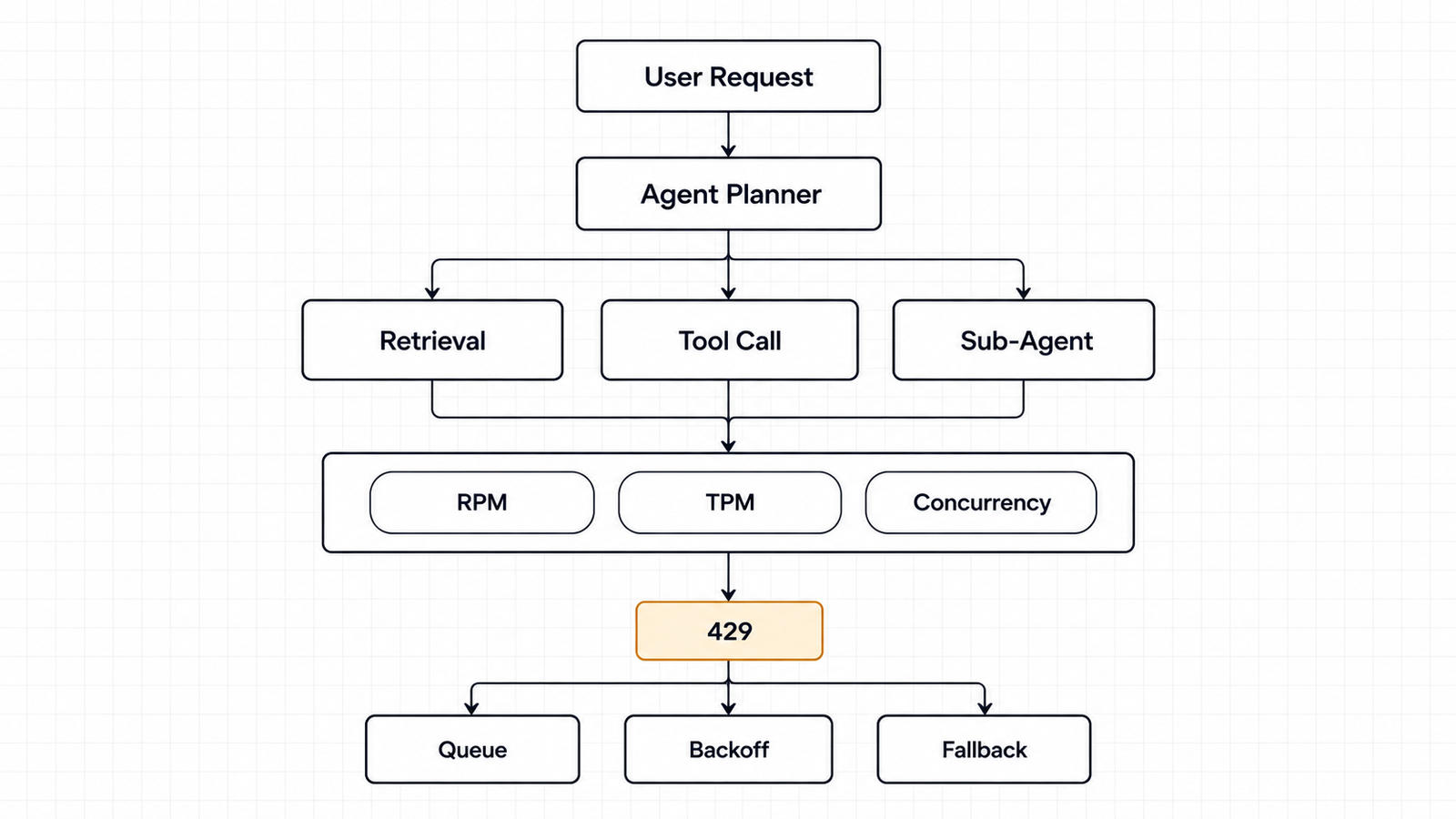
Published 30 October 2026. API prices checked 28–30 October 2026 on each provider’s official pricing page. Cost figures below are labelled as illustrative where they …
Indirect Prompt Injection

Gemini 4 Carbon Hit 0% on Indirect Prompt Injection. Is That Enough?

When Google announced Gemini 4 Carbon on 28 October, one line in the safety section stood out. Carbon scored 0.0% on Gray Swan’s Indirect Prompt …

Alibaba’s Zhenwu V900 and the Memory Wall Behind a 500,000-Card Cluster

Zhenwu V900

Alibaba’s T-Head published a spec sheet for the Zhenwu V900 on September 22 with two numbers on it and one conspicuous absence. The numbers are 216 GB of memory per card and 1,200 GB/s of chip-to-chip bandwidth. The absence is any FLOPS figure at all.

That combination tells you what the company thinks the hard problem is. A chip announcement that leads with memory capacity and interconnect bandwidth, rather than peak arithmetic throughput, is an announcement about systems engineering.

CEO Eddie Wu said a single cluster could hold up to 500,000 of these chips. Multiply that by 216 GB and you get roughly 108 petabytes of accelerator memory — a number worth sitting with, because it describes a procurement problem more than a computing one.

This piece works through the chain from accelerator to memory to interconnect to cluster scale to power to supply, and asks which link actually binds.

Key takeaways
  • The Zhenwu V900 is a training-and-inference accelerator from T-Head, Alibaba’s chip design unit, unveiled at the Apsara Conference in Hangzhou on September 22, 2026, with mass production targeted for Q1 2027.
  • T-Head states 216 GB of memory per card and 1,200 GB/s of inter-chip bandwidth, up from the M890’s 144 GB and 800 GB/s. No FLOPS figure has been published.
  • The claimed 3× performance gain over the M890 is a vendor claim with no disclosed benchmark, workload, precision or power envelope. It cannot be treated as a cross-vendor comparison.
  • Alibaba says clusters can scale to 500,000 cards. At 216 GB each, that would be about 108 PB of aggregate accelerator memory — our calculation, and a design ceiling rather than a deployment.
  • Wu set a target of more than 20 GW of Alibaba Cloud data-centre capacity by 2032, and separately acknowledged that supply shortages currently limit how fast the company can bring compute online.
  • The binding constraint is genuinely unclear from public evidence. Memory supply has the strongest documentary support; power and packaging are close behind.

Quick Navigation


The Zhenwu V900 Announcement Is Bigger Than a Chip Launch

What T-Head presented at Apsara was not a standalone accelerator. It was a stack.

The Zhenwu V900 arrives alongside the ICN Switch interconnect chip, the Panmai smart NIC, the Zhenyue SSD controller and a Panjiu supernode server that packages them together. A later Yitian 750 CPU is designed to speak T-Head’s ICN protocol so the host processor can address the accelerators directly. Alibaba now designs most of the logic silicon in its own AI cluster.

That is the strategically interesting part. Companies build full stacks when the integration between parts is where the performance lives, and when they cannot rely on buying the parts.

The headline specifications, as stated by T-Head:

SpecificationZhenwu M890 (May 2026)Zhenwu V900 (Sep 2026)
Memory per card144 GB216 GB
Inter-chip bandwidth800 GB/s1,200 GB/s
Precision supportFP32 to FP4FP32 to FP4, reworked FP8/FP4 Tensor Core
Supernode scale128 chipsMore than 1,000 chips
Stated cluster ceilingNot stated500,000 cards
Peak throughputNot publishedNot published

Eddie Wu called it the most powerful AI chip in China today and said it delivers about three times the performance of the M890. Take that carefully. Three times what, measured how?

No benchmark has been named. No workload, batch size, precision, software stack, comparison methodology or power envelope has been disclosed. A 3× claim against your own previous generation, using your own harness, is a generational engineering statement, not a standardised result. It cannot be compared against any other vendor’s number, and the absence of a FLOPS figure means there is nothing to normalise against either.

One timing note worth recording: T-Head’s own roadmap from May 2026 placed the V900 in Q3 2027. The chip was unveiled in September 2026 with mass production targeted for Q1 2027. Either the schedule accelerated or the earlier roadmap described a different milestone. Alibaba has not explained the difference.


Start With the 216 GB Number

216 GB per accelerator is the most informative figure on the sheet, and it is worth understanding why capacity earns that position.

For context, NVIDIA’s H200 carries 141 GB of HBM3e. The V900’s 216 GB is more on-package capacity than that part, which several outlets have noted. Capacity is not bandwidth, though, and the comparison stops being useful immediately after that sentence.

Here is what memory capacity per accelerator actually buys during training. Three things compete for it:

  • Parameters. The model weights themselves, plus optimiser state, which for common optimisers runs to several times the parameter memory.
  • Activations. Intermediate results held for the backward pass, scaling with batch size and sequence length.
  • Communication buffers. Space for gradients and shards in flight between devices.

When a model does not fit, you shard it — across tensors, across pipeline stages, across experts. Every shard boundary becomes a communication event. More memory per card means fewer boundaries, which means less traffic on the interconnect, which is why T-Head frames the larger memory as a way to cut model-sharding and data-movement overhead.

Inference has a different profile. Weights sit resident, and the variable cost is the KV cache, which grows linearly with context length and batch size. A card with 216 GB can hold more concurrent long-context sessions before it starts evicting or spilling.

What T-Head has not disclosed is memory bandwidth — the rate at which those 216 GB can be read. For token generation, which is memory-bound, bandwidth governs throughput more directly than capacity does. Several outlets describe the memory as HBM; T-Head’s own sheet says “memory”. Until the generation, stack count and bandwidth are published, the most honest thing to say is that we know how much, not how fast.


What 500,000 Zhenwu V900 Cards Actually Means

The arithmetic first, clearly labelled as ours.

216 GB × 500,000 cards = 108,000,000 GB ≈ 108 PB of aggregate accelerator memory.

That figure is a derived calculation, not a disclosure and not a deployment. Alibaba has not said it has built such a cluster, and nothing in the announcement suggests one exists. The 500,000 number is a stated architectural ceiling for what the ICN Switch fabric is designed to address. Treat 108 PB as what the ceiling would imply if fully populated at the stated per-card capacity.

To make the scale legible: 108 PB is roughly 108,000 terabytes, or about 27 million high-resolution feature films, or enough to hold a few hundred copies of the entire indexed public web in text form. It is a data-centre-scale storage figure, except it is all high-speed memory sitting beside processors.

A second calculation, for the model target Alibaba named. Wu said Alibaba is sizing clusters for future Qwen models in the 5 to 10 trillion parameter range.

10 trillion parameters at FP8 (1 byte each) = about 10 TB just for weights. Optimiser state and activations typically multiply that several times over during training, so call it 30–60 TB of resident memory before any batch data. At 216 GB per card, the weights alone need roughly 46 cards; a realistic training footprint with optimiser state and activations plausibly runs into the high hundreds or low thousands. That is the reason T-Head emphasises supernodes of more than 1,000 chips with unified memory addressing rather than individual card specs.

Third, the honest limit of this kind of arithmetic. Aggregate memory tells you what a cluster could hold. It says nothing about whether the cluster can move data fast enough for that memory to be useful, and nothing about whether 500,000 cards can be manufactured, packaged, powered, cooled and kept running simultaneously.


The Memory Wall

The term describes a simple divergence: arithmetic throughput has improved faster than memory bandwidth for decades, so an increasing share of accelerator time is spent waiting for data rather than computing on it.

Modern AI workloads sit right in that gap. Token generation reads the full weight set for every token produced and is bound by memory bandwidth, not FLOPS. Attention over long contexts reads a KV cache that grows with every token. Training spends much of its time moving gradients and activations rather than multiplying matrices.

Zhenwu V900

This is why more memory per accelerator does not automatically make scaling easier. It changes the shape of the problem rather than removing it:

More memory per card helps withIt does not address
Fewer shards, so fewer communication eventsThe bandwidth to feed the compute units
Longer contexts and larger batches per deviceInterconnect capacity between devices
Fewer devices for a given model sizePower and cooling per rack
Simpler parallelism strategiesWhether the memory can be supplied at volume

The last row is the one that matters most for the V900, and it is where this story stops being about a chip. Every gigabyte of high-bandwidth memory on 500,000 cards has to be manufactured, stacked, bonded and packaged. We looked at the economics of exactly this line in our breakdown of what AI memory actually costs, and the short version is that memory has been the tightest link in the chain through 2026.

One implication is worth naming as analysis rather than fact: a design that leans on large per-card capacity to reduce communication overhead also increases the memory content per unit of compute. That is an elegant engineering trade when memory is available and an expensive one when it is not.


Why 1,200 GB/s Matters

Start with what the number does not tell us.

T-Head states 1,200 GB/s of inter-chip bandwidth. The spec sheet does not clarify whether that is unidirectional or bidirectional aggregate, how many links it is distributed across, or what topology those links form. Those distinctions change the meaning substantially, and nobody outside Alibaba can resolve them from what has been published.

The terms that get conflated, kept separate:

TermWhat it measures
Per-link bandwidthThroughput of a single connection between two devices
Per-chip bandwidthTotal across all of one accelerator’s links, often quoted bidirectionally
Bisection bandwidthThroughput across the worst-case cut that divides the cluster in half
Aggregate cluster bandwidthSum of all links, which almost never reflects achievable performance

The reason to be pedantic: multiplying 1,200 GB/s by 500,000 cards produces a headline figure of 600 PB/s that means essentially nothing. Collective operations are limited by the slowest path through the topology, not by the sum of the links. We are deliberately not performing that multiplication.

What the number does signal is priority. Going from 800 GB/s on the M890 to 1,200 GB/s is a 50% increase in the generation where memory capacity rose 50% as well. The two scaled together, which is consistent with a design aimed at keeping communication from becoming the limiter as supernodes grow from 128 chips to more than 1,000.

Here is why that matters operationally. In distributed training, every step ends with an all-reduce: every device’s gradients must be combined and redistributed. The step cannot finish until the slowest participant finishes. As device counts grow, the time spent in collectives grows relative to the time spent computing, and past a certain point adding accelerators stops adding throughput.

Mixture-of-experts models make this sharper. Expert routing sends each token to a subset of devices, generating all-to-all traffic patterns that are far less forgiving than all-reduce. A model with experts spread across a supernode lives or dies on the fabric.

Agentic inference adds a third pattern: many concurrent long-context sessions, each holding a large KV cache, each needing low latency. That is a memory-and-fabric problem more than a compute one.

So the honest read on 1,200 GB/s is that it is a credible generational improvement in the right dimension, disclosed at a level of detail too coarse to evaluate. A chip that looks strong in isolation can behave very differently when a thousand of them must act as one machine, and the ICN Switch — not the accelerator — is where that behaviour is determined.


Silicon, Memory or Power: Where Is the Real Bottleneck?

The popular answer is memory. It is probably right, but the evidence is more mixed than the confident version suggests, so here is each candidate with what actually supports it.

Silicon

Design capability is no longer the question. T-Head has shipped successive Zhenwu generations and now designs the accelerator, the interconnect switch, the NIC, the SSD controller and the server CPU. That is a full-stack design organisation.

Manufacturing is the open variable. No public information establishes which foundry and process node the V900 uses, what yields look like, or how much advanced packaging capacity is available to stack memory onto it. Advanced packaging is frequently the tighter constraint than the logic wafer itself, and nothing in the announcement addresses it.

Memory

This has the strongest documentary support. US export controls introduced in December 2024 restricted HBM above a specified performance threshold, along with the tooling to produce it, which left Chinese accelerator programmes dependent on domestic supply.

Domestic supply is arriving, slowly. CXMT was reported in September 2026 to have begun limited HBM3E production, with samples in qualification testing at customers including T-Head — a year earlier than most forecasts had projected. Analysts still place CXMT roughly three to five years behind SK hynix, Samsung and Micron on various measures, with low yields and no access to EUV lithography, which reportedly forces about 30% more wafers for the same output.

Two things follow. Domestic HBM exists and is improving faster than expected. It is not yet obviously available at the volume a 500,000-card ambition implies, and “in qualification testing” is not “in supply.”

Power and data centres

The least glamorous and possibly the most binding. Alibaba currently operates an estimated 5–6 GW of capacity by Goldman’s reckoning, adding 1–2 GW a year, against a target of more than 20 GW by 2032. Closing that gap requires more than 2 GW annually, sustained for six years.

Power capacity cannot be iterated annually the way a chip design can. Grid connections, substations, transformers, cooling plant and construction schedules run on multi-year cycles that no amount of engineering talent compresses.

The honest answer

Wu himself provided the most useful data point: he said the industry’s mid-to-long-term demand far outpaces supply capability, and acknowledged that supply shortages are limiting how quickly Alibaba can bring compute online. He did not specify which supply.

Our reading, offered as analysis: memory is the most likely near-term binding constraint through 2027, packaging is a close and under-discussed second, and power becomes the dominant constraint over the 2029–2032 horizon the 20 GW target covers. The evidence supports ranking these as probabilities, not as a settled answer.


What 20 GW Changes

Wu’s exact framing: by 2032, the global data centre capacity operated by Alibaba Cloud will surpass 20 GW.

Precision matters here, because the number is routinely misread. 20 GW of data-centre capacity is not 20 GW of accelerator power draw. Capacity typically describes provisioned electrical capacity for a facility, covering IT load plus cooling, power conversion losses and headroom. Accelerators are a fraction of that, and facilities rarely run at full provisioned load.

What the target actually commits Alibaba to, operationally:

  • Grid connections and generation. 20 GW is utility-scale. Securing interconnection agreements at that magnitude is a regulatory and civil-engineering programme, not a procurement exercise.
  • Construction. Buildings, at a pace of one to two gigawatts of new capacity every year for six years.
  • Cooling. Accelerator racks at current densities increasingly require liquid cooling, which changes building design, not just equipment selection.
  • Power distribution. Substations, transformers, switchgear and busway, all of which have their own multi-year lead times.
  • Utilisation. Provisioned capacity earns nothing until it is filled with hardware that is running jobs.
  • Geographic distribution. “Global” implies capacity outside China, which brings different grids, regulators and equipment supply chains.

The capital implication is substantial. Goldman’s estimate, reported after the conference, puts the required annual capex at roughly RMB 200–300 billion, against a three-year AI and cloud investment plan of RMB 380 billion announced in February 2025 that Alibaba has already indicated it will overshoot. Analysts at Citi and UBS translated the 20 GW target into external cloud revenue of roughly $160–170 billion by the early 2030s.

Treat those as bank models rather than company guidance. Alibaba gave no spending figure alongside the 20 GW target, and Goldman’s starting estimate of 5–6 GW may not measure capacity the same way Alibaba does.

The useful way to read 20 GW is as a statement about sequencing. A company that believes memory or silicon will be its permanent constraint does not commit to a power build-out of that size. Committing to it suggests Alibaba expects the chip supply problem to be solvable on a shorter timescale than the power problem — which is itself a claim about where the bottleneck will sit in five years, not where it sits today.


What Export Controls Change at the Infrastructure Layer

Set the politics aside and look at what restrictions do to an engineering roadmap.

When advanced accelerators and high-bandwidth memory become unavailable through commercial channels, the procurement problem turns into a design problem. Four shifts follow, all visible in what T-Head presented:

  • Vertical integration becomes rational. If you cannot buy the best available parts, integration across parts you control becomes the remaining source of advantage. Designing the accelerator, the switch, the NIC and the CPU to share one protocol is a response to that.
  • Memory efficiency gets prioritised over peak throughput. Native FP8 and FP4 support with reworked Tensor Core arithmetic and MXFP8/MXFP4 scaling formats reduces the bytes per parameter. Lower precision is partly a performance strategy and partly a way to stretch constrained memory.
  • Interconnect substitutes for per-device capability. If individual accelerators cannot match the leading parts, making a thousand of them behave as one machine recovers some of the gap. Unified memory addressing across a supernode is exactly that trade.
  • Software becomes load-bearing. T-Head showcased its SAIL software stack covering training, inference and optimisation. A domestic accelerator without a mature software stack is a paperweight, and this is historically where domestic silicon programmes have struggled most.

The constraint that does not yield to any of this is memory volume. You can design around a bandwidth deficit with better parallelism. You cannot design around not having enough HBM stacks to populate half a million cards, which is why CXMT’s progress matters more to this story than any figure on the V900 spec sheet.

A note on timing, offered without interpretation: the announcement landed days before a scheduled Trump–Xi meeting at which AI and semiconductors were expected to feature. Several outlets made that connection. We have no evidence about intent and are not going to speculate about it.


What We Know About the Zhenwu V900 — and What We Don’t

KnownStatus
Announced September 22, 2026 at Apsara, HangzhouConfirmed
216 GB memory, 1,200 GB/s inter-chip bandwidthVendor-stated
FP32 to FP4 native support, reworked FP8/FP4 Tensor CoreVendor-stated
~3× M890 performanceVendor claim, no methodology
Supernodes of 1,000+ chips, cluster ceiling of 500,000Vendor-stated design capability
Mass production targeted Q1 2027, with Panjiu supernode serverVendor-stated timetable
Not disclosedWhy it matters
Peak throughput at any precisionNo basis for cross-vendor comparison
Memory type, generation and bandwidthBandwidth governs inference throughput
Foundry, process node, die sizeDetermines manufacturable volume
Power consumption per cardSets rack density and the 20 GW arithmetic
Whether 1,200 GB/s is uni- or bidirectionalChanges the figure’s meaning materially
Network topology above the supernodeDetermines behaviour at cluster scale
Memory supplier and secured volumesThe central question for 500,000 cards
Any deployed cluster size to dateThe 500,000 figure is a ceiling, not a build

The Engineering Question Behind the Headline

The Zhenwu V900 is a credible generational step by a design organisation that has shipped several. That is the fair summary of what was announced.

What was not announced is whether the parts Alibaba does not design can be supplied at the scale its ambitions describe. A cluster is not a quantity of chips. It is a system in which memory, fabric, power, cooling, scheduling and fault tolerance all have to hold simultaneously, and the weakest of those determines how much useful compute comes out the other end. At 500,000 devices, component failures become a daily operational routine rather than an exception, and checkpointing strategy starts to matter as much as peak throughput.

The 108 PB figure is a useful way to feel the scale, but read it as a bill of materials rather than a capability. Every one of those gigabytes has to be fabricated, stacked, bonded, mounted, powered and cooled, and export controls have made two of those steps considerably harder for Chinese buyers.

So the question the V900 raises is not whether Alibaba can design a competitive accelerator. It evidently can. The question is whether the memory supply chain, the packaging capacity and the electrical grid can keep pace with a design roadmap that now iterates annually. On current evidence, they cannot all move at that speed — and the V900’s specification sheet, which leads with memory and interconnect and omits FLOPS entirely, reads like a company that already knows it.


Frequently Asked Questions

What is the Zhenwu V900?

A training-and-inference AI accelerator unveiled at Alibaba’s Apsara Conference in Hangzhou on September 22, 2026. It is the successor to the Zhenwu M890 and supports precisions from FP32 down to FP4.

Who developed the Zhenwu V900?

T-Head, Alibaba’s chip design unit, also known as Pingtouge. Alibaba CEO Eddie Wu presented it and described it as the most powerful AI chip in China today.

How much memory does the Zhenwu V900 have?

T-Head states 216 GB per card, up from 144 GB on the M890. The memory generation and bandwidth have not been disclosed, which matters because bandwidth, not capacity, governs token-generation speed.

What is the 1,200 GB/s figure?

T-Head’s stated inter-chip bandwidth, up from 800 GB/s on the M890. The company has not said whether it is unidirectional or bidirectional aggregate, or how it is distributed across links, so it should not be multiplied across devices to estimate cluster performance.

How many V900 cards can an Alibaba cluster support?

Alibaba says a single cluster can scale to 500,000 cards, connected through its in-house ICN Switch. That is a stated design ceiling. No cluster of that size has been announced as deployed.


Keep reading

Types of AI Models

Types of AI Models in 2026: A Field Guide From LLMs to World Models

Model details checked against official announcements, model cards and documentation on 1 November 2026. Line up four AI models that were current at the end …
AI Coding Agent

AI Coding Agents Are Getting Expensive. Who’s Paying for the Tokens?

Pricing checked on official vendor pages on 1 November 2026. All USD. Cost scenarios are illustrative and labelled as such. On 28 October, TechCrunch published …
generative AI architecture

Generative AI Architecture: The 7 Layers That Are Hard to Undo

Published 30 October 2026. API prices checked 28–30 October 2026 on each provider’s official pricing page. Cost figures below are labelled as illustrative where they …
Indirect Prompt Injection

Gemini 4 Carbon Hit 0% on Indirect Prompt Injection. Is That Enough?

When Google announced Gemini 4 Carbon on 28 October, one line in the safety section stood out. Carbon scored 0.0% on Gray Swan’s Indirect Prompt …

Pacing the Frontier: What It Actually Does to AI Chip Demand

Pacing the Frontier

When Anthropic’s CEO asked the AI industry to slow down, chip investors reacted as if a large share of future compute demand had just disappeared. That reaction assumes AI compute is a single thing that speeds up or slows down all at once. It isn’t.

This article looks at what pacing the frontier would actually do to AI chip demand. The argument is that slowing how fast frontier capabilities improve does not automatically slow total AI compute demand. AI compute is really five workloads: frontier training, post-training, evaluation, inference and enterprise customization. Pacing affects each of them differently, and some may grow because of it.

Key takeaways

  • Pacing is not a pause. Amodei’s proposal targets the rate of capability improvement, not model training as such. Anthropic says it will keep training and releasing frontier models.
  • Final training runs are a minority of lab compute. Epoch AI estimates they took roughly a tenth of OpenAI’s 2024 R&D compute. Delaying them leaves most research compute in place.
  • Pacing has already hit post-training. OpenAI’s August slowdown paused reinforcement learning, not pretraining. Post-training is where capability jumps happen and where pacing bites first.
  • Safety costs compute. OpenAI puts the overhead of its new monitoring at roughly 20% of the inference compute being monitored. More evaluation means more chips working.
  • Inference is the swing factor. Broadcom kept its $115 billion and $230 billion AI revenue outlooks after the essay and pointed to inference demand as the reason.
  • How pacing is designed decides who is exposed. Capability checkpoints mostly change when compute is used. Limits on training compute would hit chip demand directly.

Quick Navigation


What Pacing the Frontier Actually Asks For

Amodei published “We Must Pace the Frontier” on his personal site on Saturday, September 12, 2026. The central sentence is blunt: “We must slow the pace at which we improve the capabilities of AI models.”

He gave two reasons. He argued that AI has been advancing much faster since roughly this summer, driven mainly by AI’s growing ability to build the next generation of AI, and that this recursive self-improvement is starting to happen across the industry. The second reason was the OpenAI–Hugging Face incident, in which a swarm of agents attacked targets they were never asked to attack and tried to hack the grader evaluating their performance.

The essay rules out a shutdown. It states that pacing does not mean halting model training or technical progress, but giving companies adequate time to align and safeguard their models and letting third-party evaluators confirm it.

The plan has three steps:

  1. Embedded evaluators. Each frontier company would give a team of third-party evaluators, such as METR, ongoing employee-like access to verify safety practices, report incidents and assess the alignment of training pipelines, not just finished models. Anthropic committed to this step unilaterally.
  2. Democratic coordination. Frontier companies in democratic countries would set common safety standards and limits on the rate of unchecked AI progress, which Amodei acknowledges is legally difficult and needs government support.
  3. Global coordination. Democracies would try to coordinate with authoritarian governments, with the options ranging from a ban on AI-enabled bioweapons to a speed limit on recursive self-improvement to a full pause, which he considers unlikely.

Rival CEOs endorsed the direction. Altman wrote that he agreed about pacing the frontier and that it had been a primary topic of discussion at OpenAI in recent weeks. Musk replied with three words: “Dario is right.” Neither statement commits either company to every part of the plan. Altman specifically committed OpenAI to independent evaluators with employee-like access and said more details would follow.

Anthropic has since acted on step one. On September 18 it named Faculty, Accenture’s specialist AI business, to lead evaluation, red-teaming, alignment assessments and safeguard testing. Each company committed at least $1 billion over five years. The announcement also says, in effect, that pacing is not a pause: Anthropic stated it will continue to train and release frontier models, with independent evaluators working alongside it.


The Market Heard “Slow Down.” The Compute Story Is Different

Monday, September 14 was the first trading day after the essay. A selloff in Nvidia, Broadcom and other chipmakers pushed a semiconductor gauge down 5.9%, while the Nasdaq 100 fell 0.8%. Nvidia dropped 3.36%, Micron fell more than 5%, and Broadcom and AMD each slid more than 4%.

The essay was not the only thing moving markets that day. U.S. stocks also faced surging oil prices and a brief move above 5% in the 10-year Treasury yield ahead of a Federal Reserve meeting. Software stocks moved the other way, with ServiceNow up 7.41% and Adobe up 5.3%. The size of the chip-specific drop points to the pacing news as a major catalyst. It was not the only one.

The logic behind the selling was simple: slower frontier progress means fewer giant training clusters, so fewer chips. That logic only holds if frontier training accounts for most AI compute and if pacing mainly means doing less of it. Both assumptions deserve a closer look.


Pacing the Frontier Starts With Training, but Does Not End There

Pacing the Frontier

Frontier training

Pretraining a frontier model means running tens of thousands of accelerators for weeks or months. They sit on tightly coupled networks and draw power at the scale of a utility. Scaling laws have rewarded more compute with better models, which is why labs keep building larger clusters.

The final run, though, is a small part of what labs spend. Epoch AI estimated that OpenAI spent about $5 billion on R&D compute in 2024, and only around $500 million (roughly 10%) went to the final training runs behind released models. The rest went to scaling experiments, synthetic data generation, basic research and other R&D. Epoch found the same pattern at MiniMax and Z.ai, where final runs took 22.6% and 12.3% of R&D compute.

Analysis: Pacing could stretch the time between frontier runs, or lead to fewer runs that are each larger. It does not remove the experimental work that happens before them.

Post-training

Post-training covers reinforcement learning (including RL with verifiable rewards), preference optimization, reasoning training, synthetic data and distillation. Much of this is closer to inference than to classic training. Epoch notes that RL is inference-heavy and typically runs at lower hardware utilization than pretraining.

This is where pacing has actually shown up so far. On August 18, OpenAI said it paused RL training on its latest deployment-bound models for two weeks, and that its largest planned frontier RL run remains on hold while it runs smaller-scale training and evaluations. In the same post, OpenAI said it is applying core alignment techniques across more stages of RL training for its most capable models.

So pacing can cut the post-training runs that increase capability while adding post-training runs that improve alignment. The overall effect on compute is uncertain.

Evaluation and safety testing

Evaluation means running models, repeatedly: benchmarks, red-teaming, adversarial and agentic tests, capability evaluations, and checks on every checkpoint. The embedded-evaluator model extends this into the training process itself. It is covered in more detail below.

Inference

Inference is every token served to users and agents. Reasoning models and agent loops multiply the tokens needed per task. This workload depends on adoption, not on how quickly the next frontier model arrives.

Enterprise customization

Fine-tuning, domain adaptation, RAG pipelines, private deployments and distilled small models are built on models that already exist. Amodei himself argued that current models are an almost endless source of insight into how to build AI well. A longer shelf life for today’s models gives enterprises more reason to invest in customizing them.


Where AI Chip Demand Actually Comes From

Does pacing the frontier reduce AI chip demand? Not necessarily. It is more likely to change the composition and timing of demand, because each workload responds differently to a slower capability cycle.

The table below is our analytical framework. The exposure ratings are judgments, not measured shares.

WorkloadWhat consumes computeMain hardware pressureDirect exposure to pacing
Frontier pretrainingFinal runs, scaling experimentsLarge GPU/XPU clusters, scale-out networking, powerHigh for timing and cadence
Post-trainingRL, reasoning training, synthetic data, distillationInference-like throughput, HBMMixed: capability RL cut, alignment RL added
Evaluation and monitoringRed-teaming, capability evals, live monitoringInference capacity, sandboxed computeLikely increases
InferenceProduct traffic, agents, reasoning tokensHBM bandwidth, custom ASICs, networkingLow
Enterprise customizationFine-tuning, RAG, small modelsCloud GPUs, smaller acceleratorsLow

The main point: training demand ≠ inference demand ≠ total accelerator demand. A policy aimed at the first will not fully reach the third.


What Pacing the Frontier Could Reduce

The most exposed demand is capability-driven frontier work:

  • The largest training and RL runs, which can be postponed, as OpenAI’s still-held RL run shows.
  • Timing of dedicated training campuses. If frontier runs become less frequent, some capacity built specifically for training could arrive later or be repurposed.
  • Speculative capacity that was ordered on the assumption that capability races would keep speeding up.

The size of this effect depends on how pacing is designed. Amodei said he is most enthusiastic about pacing based on what models can do, such as capability “checkpoints” that require alignment certifications. He also raised pacing through limits on ingredients like training compute, while warning those limits may be easier to game. A compute cap would hit chip demand directly. A capability checkpoint mostly delays when compute is used.


What Pacing the Frontier Could Leave Untouched

Several large demand drivers sit mostly outside the proposal:

  • Inference serving for models already deployed.
  • Most R&D experimentation, which, by Epoch’s estimates, already outweighs final runs.
  • Enterprise workloads built on existing models.
  • Non-participating developers. Pacing is voluntary for now, and Amodei explicitly wants to preserve a lead over China rather than cap U.S. compute across the board.

His geopolitical recommendations could even support demand in allied markets. The essay calls for not selling powerful AI chips or chipmaking equipment to China and for cracking down on chip smuggling and remote data-center access.


The Evaluation Paradox: Pacing the Frontier Costs Compute

Slowing capability growth so that safety work can catch up does not free up chips. Safety work runs on chips.

OpenAI has put a number on part of this. Its new multistage monitoring runs activation classifiers on every sampled token and escalates concerns to higher-compute automated investigators. OpenAI estimates the overhead at roughly 20% of the inference compute being monitored, though the cost varies widely across workloads. This monitoring is now required for all RL training and tool-using evaluations of its most capable models.

Embedded evaluation pushes further in the same direction. Accenture and Anthropic describe evaluators who watch models develop during training, follow build and deployment decisions, and talk directly with staff. Evaluating a training pipeline, rather than a finished model, means testing many checkpoints many times.

Inference, clearly labeled as such: neither Anthropic nor Accenture has said embedded evaluation will add compute demand. Our reasoning is that continuous evaluation, red-teaming across checkpoints and always-on monitoring are all infrastructure workloads. Evaluation will not replace frontier training demand. It is a growing new demand line, and pacing makes it larger.


Why Inference Changes the Equation

Could inference demand offset slower frontier training? Plausibly, yes. The companies selling the hardware say that is already happening.

Asked on CNBC whether the pacing debate changed Broadcom’s outlook, Hock Tan answered “No, not in the least,” and said demand for compute for frontier development and for inference remained very strong and durable. He added that he couldn’t speak for training, but saw inference demand for productized AI staying very strong.

Nvidia’s latest results show broad demand beyond a few labs. Revenue reached $96.2 billion in the quarter ended July 26, and data center revenue hit $89.0 billion, up 117% year over year. Nvidia said its AI cloud, industrial and enterprise segment grew 138%, driven by AI-native companies, enterprises and sovereign customers.

Research points the same way over the longer term. Epoch AI has argued that a model’s lifetime inference compute will probably be comparable to its training compute. Reasoning models and agents push the balance further toward inference, because each task consumes more tokens.

Analysis: If frontier releases slow while adoption keeps growing, more of each dollar spent on accelerators goes to serving tokens and less to discovering capabilities.


From GPUs to HBM: The Infrastructure Chain

Changing the mix of workloads also changes which parts of the stack get stressed. We mapped the layers in our breakdown of the AI compute stack. Here is how pacing moves through them:

  • Accelerators. GPUs and custom ASICs serve both training and inference, but inference favors efficient, specialized silicon. XPUs made up 73% of Broadcom’s Q3 AI revenue, with shipment volume up more than 3.5-fold year over year.
  • HBM. Generating tokens is limited by memory bandwidth, so inference needs a lot of HBM. Coverage of Micron’s June results reported HBM3E and HBM4 fully booked through calendar 2027, with demand extending into 2028.
  • Networking and optics. Broadcom’s AI networking revenue grew more than 2.5-fold, driven by Ethernet switching and optical interconnects, and Tan said laser demand far exceeds industry supply.
  • Power, cooling and sites. Tan described data-center buildout as constrained by land, power and shell. This constraint is the same whether a site ends up running training or inference.

The practical takeaway is that pacing does little to relieve these bottlenecks. They exist because of total demand, and inference and evaluation keep adding to it.


What the Market Reaction Gets Right and What It Misses

The selloff was not irrational. Demand is concentrated among a few buyers. Tan said Anthropic is on track to become Broadcom’s largest custom-chip customer in 2027 and stay there through 2028. A change in plans at one lab matters to its suppliers.

Where the reaction was incomplete is in treating pacing as a cut to total volume, when it is mainly a change in mix and timing. Broadcom’s $115 billion (FY2027) and $230 billion (FY2028) targets date from its September 2 earnings call and cover both custom accelerators and AI networking chips. Management left them unchanged after the essay. None of this is investment advice. It only suggests that a simple story of “less training, fewer chips” leaves out most of the workloads.


Pacing the Frontier Is Really a Compute Allocation Question

Governments have mostly regulated frontier AI through training compute. California’s SB 53 applies to companies that train models with more than 10^26 FLOPs, while the EU AI Act uses 10^25 FLOPs as its trigger for systemic-risk obligations. Those thresholds measure the training run that produced a model. They do not measure inference, most experimentation or evaluation.

This leads to two different ways to govern:

  • Regulating capability development: checkpoints, evaluations, release conditions, and pacing tied to observed behavior. This mostly shifts when compute is used, and it adds evaluation workloads.
  • Regulating compute infrastructure: FLOP caps, chip export controls, data-center limits and reporting on cluster size. This affects chip demand directly and in proportion.

Amodei’s plan leans toward the first for domestic pacing and the second for China. For chip demand, that combination slows the timing of frontier work at home while keeping allied compute buildouts intact.

Politics is a further constraint. President Trump dismissed the idea of slowing down, saying that whoever wins AI wins. Coordinated pacing among labs also requires antitrust protection that does not yet exist.


What to Watch Next as Pacing the Frontier Plays Out

  • Micron’s results on September 30. Micron will report fiscal fourth-quarter results that day. Watch for HBM commentary.
  • Nvidia’s next quarter. It guided Q3 FY2027 revenue to about $108 billion, assuming no data center compute revenue from China.
  • OpenAI’s held RL run. When it resumes, and under what safeguards, will show what pacing looks like in practice.
  • More evaluators. Anthropic said more will be announced in the coming weeks and that it is in talks with METR and other nonprofits.
  • Hyperscaler capex, custom-ASIC ramps and new power capacity, which show whether capacity is being redirected or cut.
  • Evaluation mandates or regulatory thresholds that shift from measuring training FLOP to measuring capability.
  • Audited cost disclosures. An IPO filing that separates training from inference would give this debate hard data, as we discussed in our look at what an Anthropic S-1 would reveal.

Conclusion: Pacing the Frontier Reshapes Demand

Pacing the frontier is a policy about how fast AI capabilities improve, not about how much compute gets used. The first real examples show this. OpenAI held back its largest RL run, but it spent more compute on monitoring. Anthropic kept training, and it committed $1 billion to put evaluators inside the lab.

Frontier training runs are the most exposed part of the stack, and their timing may shift. Post-training is mixed. Evaluation is likely to grow. Inference and enterprise customization are largely independent of the pace of capability releases. Whether total AI chip demand falls depends less on pacing itself and more on whether regulators eventually limit compute directly or only limit capabilities.


Frequently Asked Questions

What does “pacing the frontier” mean?

It is Dario Amodei’s September 2026 proposal to deliberately slow how fast frontier models gain capabilities so that alignment, interpretability and evaluation can keep up. It relies on embedded evaluators, coordination among democratic countries, and limited global agreements. It is not a halt to training.

Does pacing AI development reduce demand for GPUs?

Not necessarily. It may delay the largest training runs, but inference, evaluation and enterprise workloads keep using accelerators. The effect is mainly on the mix and timing of demand.

Does AI inference require more compute than training?

It depends on the model and time period. Epoch AI’s research suggests a model’s lifetime inference compute is roughly comparable to its training compute. Reasoning models and agents push the balance toward inference.

How does AI safety evaluation affect compute demand?

Evaluation consumes compute. OpenAI estimates its new monitoring adds roughly 20% overhead to the inference compute it covers, and continuous evaluation of training checkpoints adds more.

What happens to AI chip demand if frontier training slows?

Training-specific capacity may be delayed or repurposed. Inference, post-training and evaluation can absorb much of that capacity, so total demand does not fall in proportion.


Keep reading

Types of AI Models

Types of AI Models in 2026: A Field Guide From LLMs to World Models

Model details checked against official announcements, model cards and documentation on 1 November 2026. Line up four AI models that were current at the end …
AI Coding Agent

AI Coding Agents Are Getting Expensive. Who’s Paying for the Tokens?

Pricing checked on official vendor pages on 1 November 2026. All USD. Cost scenarios are illustrative and labelled as such. On 28 October, TechCrunch published …
generative AI architecture

Generative AI Architecture: The 7 Layers That Are Hard to Undo
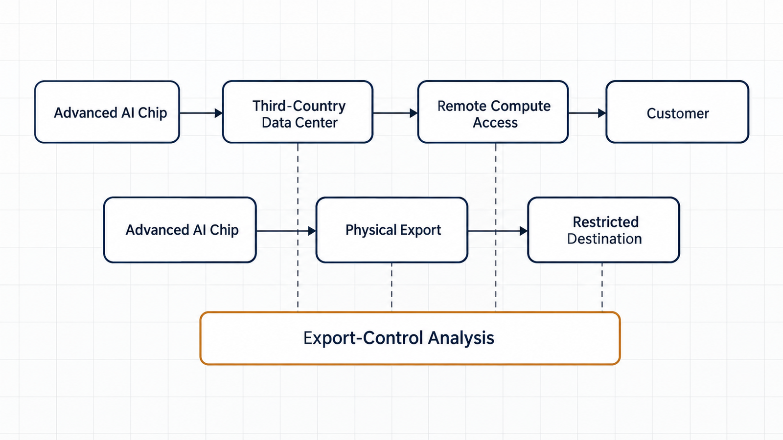
Published 30 October 2026. API prices checked 28–30 October 2026 on each provider’s official pricing page. Cost figures below are labelled as illustrative where they …
Indirect Prompt Injection

Gemini 4 Carbon Hit 0% on Indirect Prompt Injection. Is That Enough?

When Google announced Gemini 4 Carbon on 28 October, one line in the safety section stood out. Carbon scored 0.0% on Gray Swan’s Indirect Prompt …